Water Values and Hydro Offers

Disclaimer

Reasonable care has been taken to ensure that the information in this paper is up to date at the time of issue. Potential users of EMarket should, however, ensure that they evaluate EMarket and this paper through an appropriate evaluation process in consultation with Energy Link. The authors are also reliant on certain information external to EMarket and Energy Link, for which no liability or responsibility can be accepted.

Introduction

This technical bulletin is intended to provide users and interested parties with a detailed explanation of how EMarket’s water values are calculated and applied. EMarket was designed as a market simulation model rather than as an operational model and the algorithm developed by Energy Link for use in EMarket was designed to give a high degree of accuracy at high speed for this purpose. Speed of operation is a strength of EMarket and ensures that users can turn new or modified simulations around very quickly, achieving high levels of productivity.

EMarket is also a very flexible model which allows, for example, simulation runs to combine weekly, day-night and half hourly dispatches within one simulation run. This paper includes a brief overview of other features in EMarket.

Other Documents

This bulletin is one of a series of technical bulletins relating to Energy Link’s EMarket model. Taken together, the bulletins replace the old EMarket User Guide. The full series of bulletins covers an overview of the EMarket model, the details of the four major New Zealand hydro systems modelled in EMarket, water values and hydro offers, power flows, dispatch and nodal pricing, short term river chain optimisation and company optimisation.

Summary

The manager of a hydro system in New Zealand must deal with the prospect of uncertain inflows, concern about ensuring security of supply in a dry year, and how to maximise the value of water in the reservoir at any point in the year.

The concept of a marginal water value is useful in this context and defines the expected future value of the next cubic meter of water arriving in storage for generation. The water values calculated by EMarket and used in its full simulation runs are stored and viewed as water value contours, or curves of constant water value on a chart of storage versus time. Contour values are chosen to match the offer prices of thermal plant configured in each run.

EMarket’s water values have the following property: if the contour price is P_c then if the inflow scenarios entered into EMarket are projected forward until they meet the bottom or top of the reservoir then the average marginal value of water at the projection endpoints, plus any benefits/penalties on marginal water incurred along the path, will be equal to the original price.

EMarket’s water values are calculated using a much simplified, weekly version of the full simulation run which does not use full nodal dispatch and pricing, but retains the HVDC constraint. During the full simulation run the water values are adjusted using relative prices across the grid to allow for this simplified modelling and to ensure that the hydros offer their output at a price consistent with the optimum release at any particular time of year and storage value.

The offers of the major hydro systems modelled in EMarket can also be distributed optimally across injection nodes along their respective hydro systems, thus providing accurate modelling of nodal prices, losses and line constraints within and around the major hydro systems.

Water Values Defined

The concept of a water value is useful to the manager of hydro electric generation which has some storage because it tells the manager exactly how much the next MWh of generation is worth at any point in time. Knowing this, the manager could offer their hydro generation into a spot market, for example, at water value, and be dispatched more or less in order of offer price (The actual order depends also on the method used for dispatch. In New Zealand, and in many other electricity markets, nodal (or locational marginal) dispatch and pricing are used which also takes into account marginal losses and line constraints during dispatch).

Figure 1 - Water Value Contours as Operating Guidelines

Alternatively, if the manager operated an entire utility which had both hydro and thermal plant, then they could establish a place for the hydro in their "merit order", more simply the order in which the plant should be dispatched given its marginal cost of generation. The assumption here is, of course, that cheaper plant has more merit than expensive plant and should therefore be dispatched first.

Although we talk of water value, more correctly we should refer to marginal water value, which is defined as the expected future value of the next cubic meter of water arriving in storage for generation. This implies that the water value should be expressed, for example, in dollars per cubic meter of water. In practice, however, it is more convenient to express it in $/MWh of generation output.

Consequently, at any particular point in time, the hydro manager must decide if they use water in storage to generate now, or store it longer to use later. The hydro manager should take the opportunity to generate whenever the nodal price received for generation is equal to or exceeds the water value.

The marginal cost of thermal plant is made up of fuel and other variable costs of generation. Hydro electric plant has either small or negligible marginal costs, so the water value is effectively an opportunity cost – water used to generate now will not be available to generate later when we expect to obtain its current water value for generation from the hydro system.

Water Value Contours

The use of water value contours in EMarket arose from the useful concept of the operating guideline which in turn arose from the development of various models for ECNZ (Electricity Corporation of New Zealand) in New Zealand which owned most of the generation in the 1980s. An operating guideline is a curve on a chart of total storage for the reservoir in question versus time. The guideline establishes the hydro generator's place in the merit order at any given time of the year.

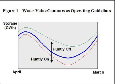
For example, the bold Huntly operating guideline shown in Figure 1, for any given time of year, gives the storage level at which the 1,000 MW Huntly power station should be operating, assuming a centrally planned system. At any time during the year Huntly should operate if storage is at or below the thick operating guideline shown. In practice, Huntly actually would come on progressively over a range of storage around the guideline. In addition, ECNZ's models calculated guidelines for all major thermal plant based on storage in the two islands, e.g. the other two guidelines shown relate to plant other than Huntly.

Another way to think of the operating guideline is a curve joining points of equal water value – in this case the average value of generation from Huntly.

Figure 2 - Typical water Value Contours for Waitaki

Thus, by definition, an operating guideline is a marginal water value contour. In designing EMarket, Energy Link decided to continue with the concept of an operating guideline because it is a useful way of visualizing how water value changes with storage and time. Water values can be represented in other ways but water value contours are highly visual and can be interpreted easily with only a little training.

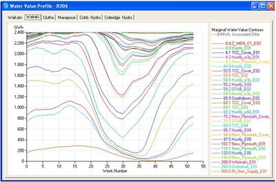
The chart to the right shows typical water value contours for water in the big storage lakes of the Waitaki hydro electric system, Lakes Pukaki and Tekapo, as produced by EMarket. Each contour relates to the offer band from a thermal generator modeled in EMarket. At any given time in the year, if storage is exactly on a contour then it is obvious what it's water value is. If storage is between two contours then the water value is linearly interpolated between the two contours. For example, if storage is one third of the way between two contours of $50/MWh contour and $75/MWh, respectively, then the water value is simply .

New Zealand Major Hydro Systems

The four major hydro systems listed below are modelled in some detail in EMarket and water values are calculated for each major hydro system.

Waitaki

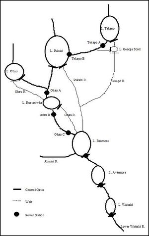
Major storage lakes Pukaki and Tekapo; inflows into lakes Pukaki, Tekapo, Ohau, and the Ahuriri River; eight power stations, some with smaller storage lakes immediately upstream.

Clutha

Major storage Lake Hawea; uncontrolled storage and inflows into lakes Wanaka and Wakatipu; other inflows from the Shotover River; Clyde and Roxburgh power stations each with small storage upstream.

Waikato

Lake Taupo with major inflows; eight power stations, each with small storage upstream, modeled downstream, of Taupo; five tributaries inflows modeled below Taupo.

Manapouri

Partially controlled storage Lakes Manapouri and Te Anau; power station at West Arm of Manapouri; outflows also down the Mararoa River.

Water values are also calculated for smaller hydro systems, e.g. Cobb and Coleridge hydro staions, if inflow data is available to EMarket.

Water Value Theory

Water value contours arise from the process of optimising the use of water in storage reservoirs upstream of one or more hydro power stations. In fact, the water value contours in EMarket allow the (simulated) hydro manager to calculate water values and simulated offers that are optimal, in a fast and convenient way.

The optimisation of a hydro generation scheme with seasonal storage is different to the optimisation of a thermal generator, which usually has access to fuel supply which effectively unlimited, for three main reasons:

1. the hydro "fuel supply," i.e. total inflows, is finite in any given year;
2. inflows into the storage reservoirs are highly volatile;
3. reservoir storage is finite.

There is one further constraint on hydro generation which is particularly important in New Zealand, where storage is relatively small compared to total inflows. The constraint is known as the "1-in-N" dry year security criterion, where N is in years. For example, the government's policy statement on electricity currently includes a 1-in-60 security criterion for dry year security of supply. In principle, this means that a shortage situation, in which demand curtailment becomes necessary or highly desirable, should only occur 1 year in 60, on average. The 1-in-N constraint is included in EMarket's water value calculations for each of the four major hydro systems modelled in EMarket.

We now ask the question - if a hydro station has operated for one year from time T₁, at which point it started out with storage of S₁, until time T₂ and storage of S₂, then what would have been its optimal set of releases at each point in the year?

The term release refers only to water released from storage to generate electricity, any other water leaving storage being classed as spill past one or more stations in the hydro system. In the following we make the assumption that generation is a constant function of release, measured in MW per cumec (1 cumec is 1 cubic metre per second). In fact, generation in MW is related to release in cumecs by a number that is approximately constant for most power stations, at least over a wide range of output. The curve relating output, g, to flow, f, through a hydro generator is given approximately by g = af - bf² where a and b are constants and the second order term in f represents frictional losses in the penstock feeding water to the turbine. In addition, a may vary with the operating head of the turbine as the lake level behind the hydro station varies – the head effect. In practice head effects are fairly small in the majority of hydro stations and usually insignificant for the purposes of the modelling undertaken with EMarket.

The time step used to calculate the water values is one week, so at some week t between T₁ and T₂ the revenue from release is given by:

[1]

where P_t is the generator's average weekly nodal spot price at time t. Total revenue for the year is given by:

[2] for all weeks between T₁ and T₂.

Marginal costs for hydro electric stations are very low, so if a hydro manager wishes to optimise gross profit over the year then they can just as easily optimise the revenue function R_tot.

A potentially important consideration is the effect of the release on the nodal price received at the node at which the generator injects, the magnitude of which may be significant if the hydro generator has market power. In practice, a higher release will often have a negative effect on the price, although for small amounts of generation this effect will usually be negligible. But to account for this possibility the nodal prices can be expressed as a function of release, P = P(r). The hydro revenue equation becomes:

[3] for all weeks between T₁ and T₂.

Figure 3 - Simple Hydro System

Before we can maximise revenue for the year we have to account for constraints on what we can achieve with our hydro electric system:

• maximum and minimum releases at each station downstream of the storage reservoirs;
• maximum and minimum storage in each reservoir;
• conservation of mass - at each step within the year the storage in any given reservoir increases by its inflows less releases and spill;
• minimum flow below stations, e.g. as set by resource consents or other conditions on the operation of each station;
• the specified 1-in-N dry year security criterion which states that the reservoir shall hit bottom only once on average in N years.

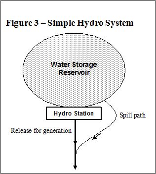
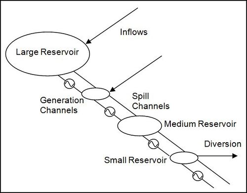
Working with a hydro system which consists of one reservoir and one station downstream, as shown in Figure 3, for the sake of simplicity, the constraints on the release are the maximum and minimum release:

[4] 0 ≤ r_t ≤ r_max for all t between T₁ and T₂

The constraints on storage are the maximum and minimum storage:

[5] for all t between T₁ and T₂

where f_t is the inflow at time t and S_min are S_max are the minimum and maximum storage.

The constraint on final storage is:

[6] for all t between T₁ and T₂

Deterministic Marginal Water Value

Using the method of Lagrange multipliers, assuming for the moment that inflows are known in advance (We refer to the inflows as deterministic rather than stochastic, the latter referring to uncertain inflows), and that we are clear of constraint conditions such as being at minimum or maximum storage, we now form the Lagrangian, , and differentiate for each r_t, which can be expressed as:

[7]

If all constraints except the binding constraint (conservation of water) given by [5] are ignored this becomes:

Equation 1: Simplified Hydro Lagrangian

[8]

This equation describes the optimal path in the absence of storage and generation capacity constraints. The remaining multiplier, L, is the marginal water value. Setting the partial derivatives of the Lagrangian to zero gives a result involving only a relatively simple differential equation:

[9]

for all t between T₁ and T₂, where L is a constant. Note that we can use the derivative of P_t rather than the partial derivative, since for our purposes P_t is a function only of r_t at each t.

Impact of Market Power

Figure 4 - Nodal Price vs Release with Market Power

It is worth noting here that dP/dr is always zero or negative and indicates the sensitivity of the market price at time t for a release of r_t. If the term is zero for all r_t then the hydro generator has no market power and is a pure price taker.

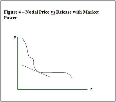
When a generator has market power then the curve relating nodal price to release might look like the complex curve shown below. The flat portion of the curve at medium and high values of r_t might represent a portion where the generator is on the margin, setting the price.

At the point shown where the tangent line intersects the curve, r_t has reduced to the point, effectively by reducing the amount offered into the market, where the generator is no longer on the margin and the price is being set by a higher priced generator. At this point, of course, dP/dr is the slope of the curve.

In the case of a generator exercising market power, it can then be concluded from the above equation that when the release is not constrained to a maximum or minimum the nodal price will be greater than the marginal water value. The r_t multiplier on the first term of our differential equation indicates that when the nodal price rises, release will be increased. If dP/dr is very small compared to P_t - the nodal price is minimally dependent on the release - then the nodal price will be more or less equal to the marginal water value and as such, constant over storage trajectories where release is not constrained.

This shows that optimal behaviour can be achieved by offering at a price that consists of a constant base price representing the marginal water value plus an additional price component that is added when nodal prices can be significantly raised by reducing release, i.e. by exercising market power.

Marginal Water Value Used in EMarket

In EMarket, the market power component of the water value equation is ignored when water value contours are calculated to give our result that hydro output should be offered each week at constant marginal water value, assuming deterministic inflows:

[10] P_t = L ≡ Marginal Water Value

In a more general sense, whether inflows are deterministic or stochastic, the marginal water value (often we refer to it just as the water value) gives us the expected future value of the next unit of water to be used to generate, given the assumptions we have made in order to derive them. In principle, the generator should generate while the price received for generation is at least the current marginal water value.

In this way, disregarding the use of market power at this stage, the behaviour of a hydro system can largely be determined by its current marginal water value. It is also worth reiterating at this point that that we are primarily concerned with the marginal value of water in long term storage reservoirs in each major hydro system. The value of water in smaller, intermediate reservoirs downstream of the long term storage reservoirs, at any point in time, could vary significantly from the value of water in the long term reservoirs - more on that in section 8.1.

Calculating Water Value Contours

To calculate water values, we must also model the reservoir manager's decision making process in the face of the considerable uncertainty about future inflows. Typically, decisions are made about the release of water from long term storage on a weekly basis. The reservoir manager knows current storage, the details of their reservoir, likewise for other reservoirs, and has some estimate of the offers made by thermal generators participating in the electricity market.

In respect of inflows, the reservoir manager knows what inflows have occurred in former years, and he knows that there is a degree of correlation in inflows from week to week.

Given this information, and armed with a technique for calculating water values for any particular inflow scenario projected forward, using equation [10], allows him to estimate the water value each week which he also knows will be updated after one week.

The Stochastic Approach

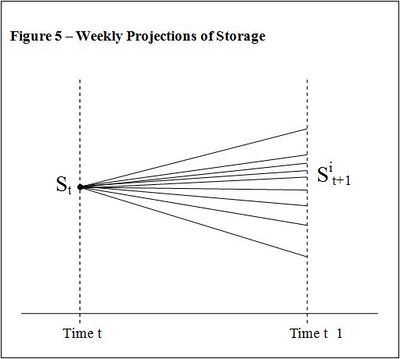
Equation [10] was derived using the assumption of deterministic inflows. But inflows are not deterministic. At any given week, t, the reservoir manager can envisage a large range of possible inflow scenarios which, when each is offered at constant water value, will each end up with a different storage value Sⁱ_t+1 at week t + 1, where i indexes the inflow scenarios from 1 to the total number of inflow scenarios considered possible.

At the end of the week, at time t + 1, each inflow scenario will take storage to a point which, in general, will have a different water value to the water value at time t. Water value is a function of time of year and storage, so let us first assume that the water values are known as a function of storage at time t, so that the final water value for each inflow scenario can be calculated.

Then using our weekly time base, and noting that the water value must give us the expected value of release at time t, the water value at St must be the weighted average of the water values given by the Sⁱ_t+1, given by:

[11]

where p(i, t + 1) is the probability (In EMarket it is assumed that all inflow scenarios are equally likely – more on this in section 6.1.) of inflow scenario i and MWVⁱ_t is the marginal water value calculated for inflow scenario i.

Figure 5 - Weekly Projections of Storage

This is the basic approach used in the RESOP module of the SPECTRA model developed by ECNZ to calculate optimised operating guidelines. RESOP finds the water value contours which have the value of the offers of the major thermal generators. RESOP was developed on the basis of using the marginal costs of the major thermal generators and the original objective of the hydro water value optimisation was to minimise the total annual fuel burn.

However, the basic result in [5] is the same whether the objective is to maximise hydro revenues over all inflow scenarios, or to minimise the cost of the total annual fuel burn over all thermal stations. This means that RESOP can be used in a competitive market environment by substituting actual or estimated thermal offers for costs. Likewise, EMarket will minimise fuel burn when thermal offers reflect fuel and other short-run marginal costs.

Adding Security

Security of supply is of paramount concern in New Zealand’s hydro dominated electricity system. But an inherent weakness of models like RESOP, which project inflows one week ahead at a time, is that they do not take account of the need to prevent the reservoir running dry in a period when inflows are low for weeks or months at a time. This is due to the fact that inflow scenarios are projected no further ahead than the end of the current week, whereas in reality hydro shortage situations develop over a period of many weeks or months.

The starting position of the water value contours in RESOP, i.e. the positions at week 52, are assumed on the first pass through the water value calculation algorithm, and so the optmisation proceeds backward in time to week 1. When the positions are known at week 1, the start of the year, these are then used as the positions at week 52 on the second pass through, and so on until the positions at all weeks converge, which usually occurs on the second or third iteration at most. Security of supply does not figure in the process described above.

In RESOP, achieving adequate security of supply is a protracted process which requires the user to produce a set of water value contours, simulate the market, determine if dry year security was achieved or not, and then adjust the offers or costs of “non-supply” generators – fictional generators added to the simulation to represent the cost of non-supply – until the required level of security is achieved.

One of EMarket’s many strengths is that dry year security of supply is built into the water value optimisation algorithm, eliminating the need to repeat time consuming reruns with different values for the shortage cost or offers for non-supply generation, to achieve the desired level of dry year security.

Figure 6 - Forward Projection of Storage

In order to determine the marginal water value for all values of storage, given any specified 1 in N dry year security constraint, it can first be observed that the marginal water value for an over-full reservoir is no greater than zero (Section 9.4 explains a recent enhancement which allows EMarket to work with spill penalties, in which case the value of water in an already full reservoir may be set less than zero). This is not to say that a generator can not spill at a price above zero, e.g. to keep the price up and maximise revenue by reducing output, which might typically occur when a reservoir is nearing full. The point here is that when the reservoir is already totally full then the marginal value of another cubic meter of water flowing into the reservoir is zero.

The marginal water value for an empty reservoir is harder to define, but when a reservoir is empty the value of an extra 1 MWh of generation, as an equivalent volume in storage, should be at least the nodal price that would occur if the hydro system's generation was removed from the market. The final marginal water value for an empty reservoir can be expressed as a shortage cost, C_S. The implied shortage cost for a reservoir in EMarket is calculated internally from the average nodal price, , for the year for the reservoir and its security factor, the number N from our 1 in N expression of the dry year security criterion. We define the shortage cost used in EMarket by:

[12]

Shortage cost tends to be poorly defined in any model that attempts to simulate it, and estimates of shortage cost vary widely. Shortage in New Zealand during dry years is partly triggered by price (e.g. large industrials with exposure to the spot price reduce production) and partly absorbed by conservation campaigns, and therefore has yet to be demonstrated in a well defined and measurable sense. EMarket’s water value calculations get around this problem by choosing water values that result in a 1 in N chance of shortage starting from the average price contour, where the user has the choice of N, the security factor. The value N is better defined than a shortage cost as 1 in N security has been a stated aim of reservoir management in the past and continues to be relevant today. Since at any point on the average price water value contour the possibility of meeting a shortage situation with the marginal water storage is 1 in N, what EMarket is doing is equivalent to simulating an shortage cost.

In essence, the shortage cost in EMarket is endogenous rather than exogenous, which is a key advantage of this algorithm, in terms of internal consistency, speed and convenience.

Of course, the user can choose to add (and usually does add) non-supply generators at strategic points on the grid. The size and price of these generators does have an impact on the implied shortage cost (and hence on ) although most of the time it is fairly small. Most users will choose the prices on their non-supply generation to act as a flag that non-supply has occurred and perhaps also to be some proxy for an exogenous shortage cost. But their choice is also likely to be made to give spot prices in the event of a very dry year which represent where they believe the market might actually go during such an event.

Given a marginal water value at any time of year, a projection of future dispatches and inflows can be made using forecast demand (Note that EMarket does not model demand elasticity in the forward simulation phase), offers from other generators and the input inflow scenarios. A different projection will be made for each inflow scenario. For a given starting storage, and its water value, a certain number of these projections will eventually reach maximum storage and the others will eventually hit the bottom of the reservoir - this typically happens within just a few months in New Zealand’s storage reservoirs. Since optimal releases are based on a constant marginal water value in between the two storage limits, the average resulting value of the marginal water should be equal to the starting marginal water value. This is the criterion used by EMarket for determining marginal water value's.

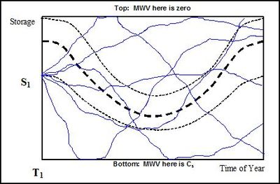
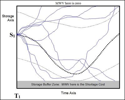
The figure below illustrates how this works, though it must be noted that EMarket does not use this method of projecting storage forward to actually calculate the water value contours – the method is described in section 6. The figure shows storage versus time of year starting from time T₁ and projecting forward for a number of annual inflow scenarios. The dashed black lines are water value contours, and storage at T₁ is equal to S₁ which is on a water value contour. The thin solid traces are the result of dispatching forward with the different inflow scenarios. Most inflow scenarios meet one or other storage constraints within a few months.

Every inflow scenario that hits the top of the reservoir, resulting in spill, must have had a marginal water value of zero, given our result that constant marginal water value is optimal - refer equation [10]. Every inflow scenario that hits the bottom of the reservoir, resulting in shortage, must have had a marginal water value of the shortage cost, C_S. If n inflows scenarios hit bottom then the marginal water value at S₁ is given by:

[13]

where F is the number of annual inflow scenarios entered into EMarket.

Thus, the marginal water value at S1 is equal to the average of the marginal water values of all inflow scenarios at their respective end points at either maximum or minimum storage. The position of the contour at time T₁ is obtained by adjusting the contour position until the average water value over all inflows is equal to the price of the contour. Note that all F inflow scenarios will hit either the top or bottom of the reservoir, usually within a few months.

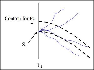
To illustrate how the water value contours behave, suppose that water value contours for a major hydro system have been calculated for a particular simulation run and at the point at S₁ and T₁ is as shown in Figure 6. Now suppose that the demand input for the run are changed so that demand for the same run is now higher than previously – what happens to the water value contours?

Projecting forward from S1 with higher demand, all other things being equal, will most likely result in greater dispatch of the hydro system. Hence one or more of the inflow scenarios that previously hit the top of the reservoir before hitting bottom will now hit bottom first - let us suppose that just one inflow scenario is affected in this way. As a result, equation [13] will give us . The contours are chosen to have values which are equal to thermal offers set up in the simulation run, so with the lower demand we must have had that MWV = P_c, where P_c is the offer price associated with the contour.

But our new water value is higher than it was previously so our point S₁ at T₁ can no longer be on the water value contour for P_c, since P_c has not changed – only demand has changed in this example. The point at S₁ and T₁ shown in Figure 7 now has a water value greater than P_c, so the water value contour for P_c has moved up at time T₁.

This example shows that increasing demand will tend to move water value contours up relative to storage, though the amount depends on a number of factors in each case. With a little practice, users can also learn to quickly “read” water value contours and predict changes to water value contours.

While this section has illustrated how EMarket calculates water values, the calculations are not actually done in this way, and a shortage cost does not need to be calculated, though the end result is the same. An advantage of using projections that hit either the top or the bottom of the reservoir is the ability to include the 1-in-N security criterion directly in the calculation of water values. This method also captures the full impact of serial correlations within inflows.

The Average Nodal Price

is the average over F inflow sequences and 52 weeks. It is derived by running the simulation until it converges, so it is sensitive to the security factor, which in turn ensures that shortage costs are N times the average price. If during a simulation shortage costs appear too low, then the security factor can be increased to reflect expectations.

EMarket’s water values are based on historical inflows as they occurred. In contrast, RESOP and some other models treat inflows and reservoirs as independent, e.g. RESOP models water values using storage on other reservoirs over a grid covering the total range of storage. As a result, RESOP’s water values probably go much higher than EMarket’s in the event that Waitaki storage gets very, very low or even empty – in this event all other reservoirs would also be empty or near empty.

In practice, borne out by countless simulations and the market itself, getting storage this low in the Waitaki is highly unlikely. For starters, demand elasticity typically kicks in well before Waitaki runs out. In EMarket, Waitaki also includes the Low Buffer inputs (refer section 6.6) which puts the bottom of the reservoir (for the purpose of calculation of water values) above zero storage – a Low Buffer of 300 GWh would be typical. The result is that in EMarket the Waitaki never gets into that low region of storage where, when the other reservoirs are empty, water values increase exponentially. Therefore, borne out by the market itself, the loss of accuracy in EMarket’s water value is negligible.

Calculating the Marginal Water Values

EMarket contains four major hydro systems for which contours must be calculated, after which the contours for the small hydros are calculated - this discussion focuses on the four major hydros. Because of the time it takes to make a full multi-dimensional estimate of marginal water values as a function of the storage at all four major systems, EMarket first calculates the marginal water values for the major hydro reservoirs given that there is no knowledge of the storage in other reservoirs.

The aim of the calculation of marginal water values in EMarket is to determine the position of marginal water value contours that correspond to the prices of offers from the non-hydro offers included in EMarket simulation runs, thus producing the familiar water value contour curves, the analog of ECNZ’s original operating guidelines. This leads to a method that is fast and produces results that converge quickly and accurately.

The algorithm used has two stages, which are applied in successive iterations for each major hydro system: simulation (This is not the same as the detailed simulations of the system that are actually run using the water values once calculated. These simulations are on a weekly basis and undertaken only for the purpose of calculating the water values) and contour calculation. For the purposes of both stages, a simplified dispatch of generation offers is used which stacks offers in order of price but also constrains maximum generation on each island according to the constraints on the HVDC link. The simplified dispatch includes a fixed allowance for losses on the grid, currently set at 3% for New Zealand.

In the following sections we will assume that weekly average historical inflows are available to EMarket covering the period from April 1931 to March of the last inflow year used as an input (“the last March”). The total number of inflow scenarios entered is given by F, currently in the high 70s, but in general will adjust to the number of complete April-March scenarios entered into EMarket for any particular simulation.

Simulation Stage

The first stage is a simulation of the entire system over all inflow years. Each of the four major hydro generators offer in a way which simulates how the run is actually set up in order to get accurate water values:

• must run is offered at the must run price set up for the major hydro;
• inflows into controlled reservoirs and tributary inflows are modelled separately;
• the remaining generation is offered at marginal water value, which is determined by standard seed marginal water value contours (These are set internally within EMarket based on experience in running simulations. The speed of convergence is not particularly sensitive to the seed water values used) – time of year and storage in the reservoir at each weekly step in the simulation;
• if a hydro reservoir reaches maximum storage it offers over-full storage in at a price of zero. When storage gets low, maximum generation is cut accordingly;
• details of the major hydro systems are modelled to a reasonable degree, for example the bypass that would have occurred with the new stations forming the cancelled Project Aqua on the lower Waitaki is modelled explicitly during this phase.

The simulation runs continuously through all F inflow years so that the starting storage for year n is the final storage for year n – 1. It starts with two mean years to get accurate starting storage for April 1931 and then proceeds through to the last March.

All other offers entered into EMarket, those from thermal stations and other stations that are simulated as operating to a generation profile, are calculated based on an assessment of how the offers vary over the year. Offers may vary based on time or based on other factors programmed in the EMarket Schedule described briefly in section 10.

The offer quantities, prices and spill are all recorded for the entire set of historical inflow scenarios available to EMarket. These results are used solely to provide the contour calculation phase with a realistic set of generation quantities to work with for all weeks and inflow years - in a wet year more must-run offers will occur and in a dry year generation may be limited from some systems.

At this point we also have an array of prices by week which allow us to calculate the average price for each hydro over all inflow years, which we denote just as for simplicity – each major hydro actually has a different value for .

Contour Calculation Stage

In principle, each contour's position could be calculated for each week using the method of forward projection illustrated in section 5.4 and Figure 6. However this would be time consuming, so a faster dynamic programming method is used which also does not require the shortage cost, C_s, to be calculated.

To obtain our water value contours the contour prices, P_c, are chosen to be those of the thermal offers entered into EMarket and used in the simulation phase. The contours are calculated for each hydro system in turn. Let us suppose we are on the first hydro system and contour c, by which we mean that it is the c^th lowest offer set up in the simulation, with thermal offer price of P_c.

The market is simulated from April 1931 to the last March with the first major hydro system offering discretionary output above must-run at P_c. This offer is dispatched against the thermal offers and the generation quantities calculated for the other hydros in the simulation phase. The output taken from this simulation of all F inflows scenarios is a set of weekly changes in storage, ΔS_t for t = 1, ..., 52, for each and every inflow year (Giving a total of 52 × F ΔS_t's. Each ΔS_t is specific to its week and inflow year), for the first hydro system.

It is important to note that all this simulation does is work out dispatch and inflows for every week in the sequence with the reservoir unconstrained, i.e. there are no full or empty constraints on the chosen hydro system during this simulation. The constraint on maximum generation from a hydro scheme remains in place, however, so that when demand cannot be met, ΔS_t will reflect maximum release. In practice, most EMarket users include non-supply generators in their simulation input data so the chance of demand shedding occurring in the forward simulation is usually small.

Figure 8 - Forward Projection - Calculation of the ΔS_j

Backward Projection

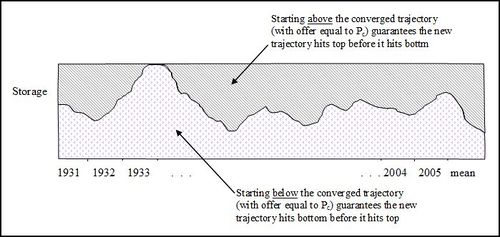
Although the concept of water value contour is best illustrated using diagrams like that shown in Figure 6, the method used to calculate the contours is considerably more efficient when backward projection is used. For the contour with price P_c the aim of the backward projection is to produce a single, converged storage trajectory spanning F + 1 years, in such a way that if another trajectory is created by projecting forward with constant water value P_c but starting above the converged trajectory, it is guaranteed to hit the top of the reservoir before it hits the bottom. Likewise, starting below the converged trajectory guarantees the new trajectory will hit the bottom of the reservoir before it hits the top, as shown in the figure below.

Figure 9 - Backward Projection

The ΔS_j are now used to project storage backward, starting at the final storage for March 2003 just calculated. This process runs backward from March of a mean year to April of a mean year (A mean inflow year is a year mean weekly inflows, so the inflow in each week is simply the mean of all F inflows for the relevant week), then end-to-end into the last March and then end-to-end back to April 1931. The storage at April 1931, after processing back F + 1 inflow years end-to-end, is then used as start storage for April of the mean year for a repeat of the simulation, thus reducing the impact of assumptions about starting storage.

This process is a form of optimisation known as dynamic programming since it starts at an optimum storage position and works back from that assuming the optimum offer strategy is to offer at constant marginal water value.

Figure 10 - Converged Trajectory Dividing the Reservoir

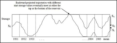
The next figure shows a 74 year backward projection of storage for a given contour value P_c for a given major hydro reservoir, but starting at two different storage values S_u and S_l. The two trajectories follow different paths for a while, but eventually meet at either the top or the bottom of the reservoir. To the left of this point, as indicated by the arrow in Figure 11, the trajectory splits storage into our two required regions – refer Figure 10. But to the right of this point the region between the two trajectories contains the point from which storage could hit top and bottom of the reservoir when projected forward.

Hence EMarket runs through the backward projection twice, using S₀ as the starting storage the second time, so that the trajectory converges throughout its length.

Figure 11 - Converging a Backward Projected Trajectory

Properties of the Backward Projected Converged Trajectory

Figure 12 - Backward and Forward Projected Trajectories

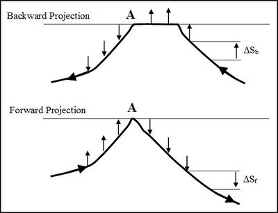
It is not immediately obvious from Figure 10 why any forward projected trajectory that starts above the converged trajectory shown will hit top before it hits bottom, or vice versa. The key to understanding this is to consider the differences between backward projection and forward projection, and we do this by studying the left-most point in the figure at which the trajectory hits the top of the reservoir, as shown in Figure 12.

The converged backward projected trajectory at the top of the figure is formed by projecting backward using the weekly changes in storage, ΔS, but because we are projecting backward the ΔS_b have opposite sign to the original set. When this trajectory hits top the ΔS_b are spilled until their sign changes and the trajectory leaves the top of the reservoir at A.

The lower trajectory is forward projected, so now the ΔS_f have the same sign as the original set of storage changes and opposite sign to the ΔS_b. The forward projected trajectory is started at the same storage as the backward trajectory finishes at, but when this trajectory hits the top of the reservoir at A, at the very next week it leaves the top of the reservoir - it just grazes the top of the reservoir at A.

We can now see that if this forward projected trajectory starts at any lower storage value it will not reach the top of the reservoir. It is also obvious that if the starting storage is higher then it will still hit the top of the reservoir. Hence we have shown that the converged backward projected trajectory splits the storage chart into the two zones shown in Figure 10.

Contour Selection

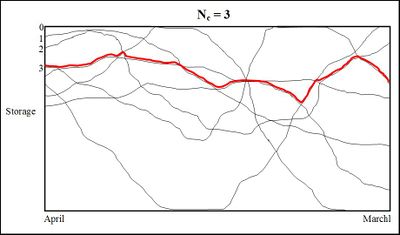
The F year converged backward projected storage trajectory – April 1931 through the last March – is then split into component April-March years and put onto one “chart” as shown in Figure 13.

Before choosing the water value contour, we recall that 1 in N security is required for dry years. The price of this contour is P_c and so, combining [12] and [13], the security associated with this contour is given by N_c where:

[14]

which is to say that the number of inflow scenarios that empty the reservoir starting from this contour is N_c. A corollary of this is that if the water value is equal to and if F = N then the number of inflow scenarios which will hit bottom of the reservoir when projected forward using market dispatch and constant offer price , is equal to 1.

Figure 13 - Contour Selection

Starting at zero for the $0/MWh contour at or very near the top of the reservoir, at any week in the year, we can count down the storage trajectories on the chart below. The number of the contour corresponding to offer price P_c is numbered N_c. For example, if P_c = $145.95/MWh, F = 74, = $60/MWh, N = 60 (for 1 in 60 security of supply) then N_c = 3 and the required contour is therefore given by the third trajectory below the zero contour (at the very top of the reservoir) in each week.

In Figure 13 the top of the reservoir is the contour for $0/MWh. The bold red line follows the third storage trajectory down from the top of the reservoir at each point in the year – in our example this is the contour prices at $145.95/MWh. (Note that the bold line is drawn slightly above the third trajectory down for the sake of clarity.)

The bold red line is made up of storage values at each week such that the average outcome over all inflows projected forward, either spill or shortage, is equal to the contour price, our condition for optimality. Above the contour, more inflow scenarios will result in spill and less in shortage, and vice versa below the contour.

Consider for a moment the first week in the April-March year. The backward projected trajectories split the reservoir into two zones, so any of the three trajectories numbered 0 – 2 that have their first week values above the third trajectory down, if moved down to start at the April starting point of trajectory 3 (shown above as ‘3’), on a forward projection, must hit bottom before they hit top when projected forward.

Likewise, any of the F – 3 trajectories below the third trajectory down, if projected forward starting at 3, must hit top before they hit bottom. Thus the bold red line defined by the third trajectory down at each week gives us the water value contour for Pc. Equation [13] gives us:

[15]

This process is repeated for all contour values P_c to give the first set of new water value contours for the first hydro system. The next step is to repeat the simulation phase outlined in section 6.1 above to calculate a better set of generation quantities to use in the contour calculation phase for the second hydro system.

The process described for the first hydro is then repeated for all other hydro systems until EMarket has a full, new set of water value contours for all hydro systems. The entire simulation-calculation phase is repeated three times which ensures that contours converge without excessive computation.

At this point EMarket is ready to run the actual simulation.

Non-integer Trajectory Number

Figure 14 - Contour Selection with Non-integer Trajectory Number

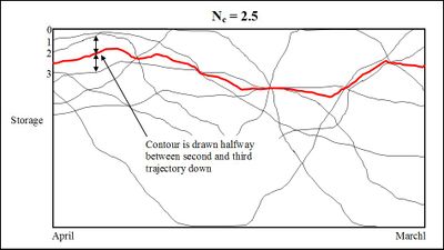
When N_c is found to be non-integer, it could just be rounded off to the nearest integer. But EMarket actually interpolates between adjacent contours in order to achieve higher accuracy. For example, if N_c = 2.5 then the contour will be chosen to be the storage level which is halfway between the second and third storage trajectories down from the top of the reservoir.

Implied Shortage Cost for a Reservoir

In section 5.4 we defined the shortage cost for a major hydro generator as N times the average nodal price over the simulations undertaken to calculate the contours, , where N is the security factor defined by the 1-in-N security criterion.

Using our method of backward projection, the shortage cost does not need to be calculated in EMarket, but it is necessary to define it so that we can construct the water value contours we require – those that maximise hydro revenue without recourse to market power while also maintaining any specified level of dry year security.

The method of construction of the contours means that whenever storage for a major hydro system is on the contour for the average nodal price(There may not be a thermal offer equal to the average nodal price, and hence no contour calculated in EMarket for this value, but the point is that it could be calculated), , then from that point only one input inflow sequence will take storage to the bottom of the reservoir when projected forward. In the case of the Waitaki system bottom of the reservoir means the top of the Low Buffer entered by the user – refer section 6.6 below. Although this construction is somewhat arbitrary, it is nevertheless a reasonable interpretation of the requirements around dry year security.

As the price increases above the probability of shortage increases above 1-in-N and vice versa.

Waitaki Special Parameters

Figure 15 - Forward Projection of Storage with Waitaki Low Buffer

Due to the critical importance of the storage in the Waitaki hydro system, principally storage in lakes Pukaki and Tekapo, EMarket contains special parameters which relate only to the seasonal storage in Waitaki.

Figure 6 shows how inflows projected forward hit either the top or the bottom of the reservoir quite quickly. Figure 15 shows the actual modelling of the storage in the Waitaki system. A storage buffer zone, an input into EMarket, allows for the fact that extra measures will be taken by hydro companies to avoid shortage once shortage becomes likely. A buffer size in GWh is entered as the 'Low Buffer' input for the Waitaki hydro system only. The bottom of Waitaki’s seasonal storage is taken as the top of this buffer zone.

Once storage is in this region then Waitaki takes action to reduce releases, reducing the maximum output by a set MW per GWh ratio entered as the 'Reduction Ratio'. The effect of this is to scale down releases as storage falls within this buffer zone which. For calculation of Waitaki's water values in EMarket, the top of the Low Buffer region is taken as zero storage. The buffer zone can be thought of as Waitaki’s “no-go” zone – Meridian Energy would effectively never want storage to get this low because the risks around having to buy from the spot market when prices are very high in an extreme dry year are huge (The Waitaki Low Buffer is often set to 300 GWh, however there is some evidence, gleaned from observation of the market, that Meridian operates to an even greater buffer than this).

Accuracy of Water Values

The water value algorithm in EMarket is a version of stochastic dynamic programming, designed to work both quickly and accurately in New Zealand’s highly constrained hydro-dominated electricity supply system along with nodal dispatch and pricing.

To ensure the preset 1-in-N dry year security criteria is met, storage is projected forward for each inflow scenario at constant water value at each week in the contour calculation stage until they hit either the top or the bottom of the reservoir – refer to section 5.4. But the same projection undertaken in the full simulation runs in EMarket sees the water value change at the start of each simulated week as storage changes relative to the water value contours, apparently in contradiction to the projections undertaken when the contours are calculated.

The question thus arises - how is this contradiction manifested in the full simulation runs and how does it impact on the accuracy of the water value contours?

The answer is that, within the limits of the accuracy of the weekly simulations undertaken to calculate the water value contours, a high degree of accuracy is obtained. The explanation has two parts. Firstly, the security criterion typically in use in New Zealand is relatively stringent, and the historical inflow records show that only a small proportion of extremely dry inflow scenarios have an influence on how the criterion is met.

Secondly, the extremely dry scenarios are so much drier than the majority of inflow scenarios over a sustained period that they tend to determine the shape of the water value contours at higher prices - these are the contours that act to curtail hydro generation, relative to other generation, when the risk of shortage rises to higher levels. Thus, the shape and position of the contours that really drive security of supply are significantly more sensitive to the extremely dry inflows than they are to the water values assumed during forward projections of inflows.

Dry Year Security for Waitaki

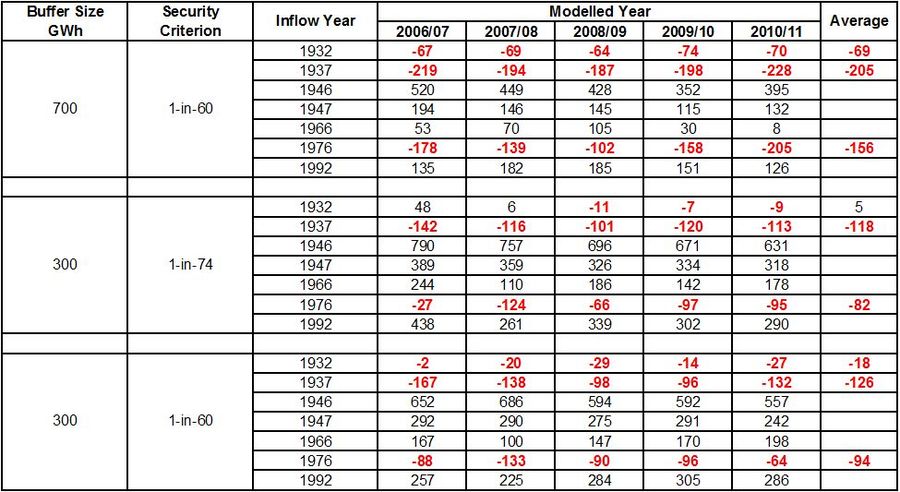
The most important hydro system for preservation of dry year security of supply is the Waitaki system in the South Island, partly because of its location in the South Island but primarily because it is the largest reservoir in the country by a large margin. Tests on EMarket’s performance in respect of security show that its water values preserve the required 1-in-N level very accurately, providing of course that the inputs in the simulation runs are not too different to those prevailing during the water value calculations. For example, test runs based around market and demand scenarios for the five years 2006/07 – 2010/11 gave the results in Table 1 below.

The results are taken from the fully detailed simulation runs in EMarket which use the water value contours, and not from the simplified simulations undertaken solely for the purpose of the water value calculations, described in section 6.1.

The table shows the driest inflow scenarios on record and the bold red values are the storage amounts, expressed in GWh, that each scenario enters the low buffer zone set for the Waitaki system, so a negative value indicates that the buffer is entered.

With 1 in 60 security we would ideally expect 1 or 2 scenarios to graze or enter the low buffer zone. In each of the 1-in-60 cases above three scenarios enter the low buffer zone. If we take the error as being the amount the third highest scenario enters the low buffer zone then the average error would be between 18 and 69 GWh. These figures equate to 0.8% and 2.9% of the total size of Waitaki’s seasonal storage reservoirs, or 9.9% and 6.0% of the low buffer in each case, respectively.

Table 1 - Low Buffer Entry Values for Dry Years on the Waitaki

For the 1 in 74 case we would expect only one scenario to enter the low buffer, although based on the average errors shown there are actually two that enter with the average error on the highest of the two scenarios being 94 GWh.

The errors occur due to differences between the detail to which the electricity supply system and market are modelled in the water value calculation phase versus the full simulation phase. To achieve higher accuracy would require that the simulations undertaken only to calculate water values be significantly more detailed, particularly in respect of the dynamic modelling of losses and line constraints on the grid.

Small Hydro Generators

There are a significant number of small hydro systems around New Zealand which may be configured in EMarket as hydro systems and optimised with their own water values. They are calculated in the same manner as described above for the four major hydro systems, except they are calculated only once water value contours are completed for the four majors. Note that this only applies to the small hydros for which inflows are entered into EMarket.

During the calculation for the four majors the small hydros are assumed to generate their average output based on the inflows entered into EMarket for these small systems.

Comparison with Other Water Values

EMarket projects inflow scenarios ahead until they either hit the top or the bottom of the reservoir, which typically happens within a few months at most. The three great strengths of this approach are that:

1. the water values maximise revenue (or minimise the cost of total fuel burn if thermal offers are based on short run marginal costs) given uncertainty in inflows;
2. dry year security is achieved without the need to revert to time consuming reruns and assumptions about shortage costs;
3. the impact of longer and shorter term serial correlations in inflows are captured in water values.

Other models in use in New Zealand do not combine these three strengths while, at the same time, running very fast and accurately.

Deterministic models such as PLEXOS (The comments about other models are based solely on analysis of the publicly available documentation on these models) assume that inflows are known in advance and may simulate overly optimistic operation of hydro schemes. Other models which do optimise water values with uncertain inflows do not contain the dry year security constraint within the optimisation, and treat inflow scenarios differently, as discussed in the following section.

Inflow Scenarios

Inflows are entered into EMarket via one or more csv files which include inflow years by week, the units being average weekly cumecs. The usual approach to inflow scenarios with EMarket is to work with the set of available and complete historical inflows, typically dating back to the 1920’s or 1930’s in the case of the major hydro systems in New Zealand (Energy Link can supply inflows with EMarket or the user can obtain their own inflows from other commercial sources).

But it is recognised that the historical record is relatively small and that current trends in inflows may not match the data in the historical record, e.g. due to climate change or due to long term climate cycles. Users may therefore enter alternative sets of inflows into other csv files and easily configure EMarket to use these.

For example, a set of 500 synthetic inflow years could be created using an alternative inflow model and provided to EMarket to work with. The choice is entirely that of the user.

This paper is not intended to fully canvas the many issues around inflows, however there are a number of points to note about inflows that are key to understanding why EMarket’s water values are calculated in the way they are and the potential impact on results, regardless of model used, depending on how inflows are used.

Using Figure 6 to help us visualise how EMarket works with inflows, we see that the input inflow scenarios are projected ahead until they hit either the top or bottom of the reservoir, thus establishing an expected water value at time T₁ and S₁. This method places a high degree of emphasis on the complete input inflow scenarios, which are more often than not historical inflow scenarios.

However, models such as RESOP and SDDP, the latter also in use in New Zealand at present, project only one week ahead at a time, as shown in Figure 5. This means that these models effectively work with a much larger number of inflow scenarios. For example, if there are 74 historical annual inflow scenarios input by week then the implied number of scenarios, using a 52 week year, is 74⁵². In New Zealand, the average inflows over a period is critical, especially the period from January through June when, on average, inflows peak and then fall off to a minimum going into winter, at the same time as demand increases toward the winter peak.

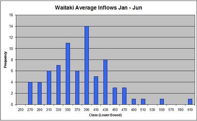
In EMarket, using historical weekly inflows, there are 74 scenarios for Jan-Jun inflows, whereas in weekly models which treat weekly inflows as independent of each other, working with an equivalent 26 week period, 74 historical inflow scenarios would imply 74²⁶ inflow possible inflow scenarios. In this case the minimum average inflow for the period would be 156 cumecs and the maximum 1,215 cumecs, compared to the actual minimum and maximum average inflows of 277 and 612 cumecs, respectively.

The central limit theorem states that the distribution of the sum of a number of random variables tends towards being a normal distribution. Given that 74²⁶ is a very large number, we would expect the implied distribution of inflows to be normal. Figure 16, however, shows the actual distribution of average inflows into the Waitaki catchment (Includes inflows into lakes Pukaki, Ohau and Tekapo, plus tributary inflows into Lake Benmore) over 74 years of inflow data in 20 cumec classes.

It has been suggested (Refer to Econometric Modelling, W H Greene, Prentice Hill) that a method for testing whether the distribution underlying a sample is normal is to refer the statistic

[16] sample_size[skewness² / 6 + (kurtosis - 3)² / 24]

to the chi-squared distribution with two degrees of freedom. The data shown in Figure 16 this statistic evaluates to 11.0 which has a probability of less than 0.5% - the test would say that the distribution is normal with less than 0.5% probability.

Figure 16 - Waitaki Inflows January - June

This test, although based on a small set of inflow data, tends to back up visual inspection which is consistent with something other than a normal distribution. Jan-Jun average inflows in the historical record have a distinct lower bound at around 280 cumecs. At the high end, the distribution exhibits a long and significant tail.

Weekly models such as RESOP and SDDP recognise that there is serial correlation (correlation week to week) in inflows and make adjustments for this. For example, SDDP makes an adjustment based on a correlation from one week to the next, so the impact of the correlation dies out quite quickly. The historical inflow data suggests that correlations could be significant across much longer periods.

This is by no means a comprehensive review of the underlying distribution of inflows in the critical period from January through to June. However it does raise two important of issues:

1. weekly models, unless they correctly capture the serial correlation, are in danger of treating inflows as if they are normally distributed;
2. if the correlation is not adequately captured then the weekly models are in danger of converging to deterministic inflows, possibly accounting for anecdotal evidence suggesting that shortage costs must be set very high in these models to achieve adequate levels of dry year security, avoiding non-supply or demand curtailment.

When weekly models are used to calculate water values, the ultimate test of these is generally to run detailed simulations against the water values to check if dry year security is maintained, but using the driest inflow scenarios from the historical record. In other words, despite their construction, the ultimate dry year security test for weekly models is how they handle historical dry years.

In EMarket, assuming that historical inflows are input, the water values directly reflect the critical dry year security criterion, which is based on historical dry year inflows. In addition to this direct linkage with the all-important dry year management, EMarket’s water values also avoid building characteristics into modelled inflows that are not present in the inflow scenarios used as inputs into any particular simulation with run with EMarket.

Multi-reservoir Effects

The water values in EMarket for each major hydro are calculated with respect to storage in the reservoir concerned, without direct recourse to the storage in the other major reservoirs. It is conceivable that this could result in excessively cheap hydro generation being offered when all systems are running low, even though they all face a greatly enhanced probability of shortage. It should be noted that this effect would be likely only if all reservoirs were at extremely low storage, i.e. near empty.

However, tests indicate that the marginal water value at Waitaki tends to be a function of total storage in the country and that marginal water values at the other reservoirs are more or less independent of this except for when total storage is very low. Assuming the burden of dry year security lies with the Waitaki system, it appears from our work that this system can behave almost independently and will carry all the vital storage for the other systems. This is what occurs in all simulations of the algorithm described above so it appears that enhanced shortage costs can be isolated to the Waitaki system without loss of generality.

For example, if Manapouri were nearly full when Waitaki was empty, then the marginal water values for Manapouri calculated in EMarket could cause it to offer too cheaply. However, typically what happens is that other lakes empty out before the main Waitaki lakes, matching what is implemented in EMarket. Observations of the market over a number of years confirm that Waitaki is operated in such a way that storage never gets into the very low region. This is reflected in EMarket by the presence of the low buffer on the Waitaki system which is typically set by users to between 300 and 750 GWh. When Waitaki storage is in the low buffer zone Waitaki offers progressively less as storage falls.

It must also be noted that the optimisation of water values does not explicitly account for unexpected outages of major plant, surges in demand, or line outages, so prudent operation of Waitaki in particular, necessitates allowance for a storage buffer in case of such an eventuality. This is another reason to use the low buffer zone.

Similarly, when a reservoir is full EMarket includes an input parameter for Waitaki which allows water values to reduce earlier in order to avoid spill.

Application of Water Values

In this section we review how water value contours, once calculated, are actually used in the full simulation runs which produce the output data which users actually view, process and report.

Hydro Offers in EMarket

We have seen that the manager of a hydro generator with storage should calculate the marginal water value, which turns out to be a function of time of year and storage, and in principle offer all releases at that price. EMarket calculates the water value contours in one go for an entire year, after which the water value can be looked up week-by-week during any simulation run. By virtue of the method used in EMarket, the water values include the cost of providing the specified dry year security criterion setting in each of the four major hydro systems.

In practice, hydro stations have a more complex offer structure than indicated simply by examining water value contours, and this is mirrored in EMarket. For example, a minimum flow requirement at a station will be offered as must run, which means the generator output that achieves the minimum flow will be offered at a low price to ensure dispatch.

Figure 17 - Structured Waitaki Offers

Offers above must run in EMarket reflect water values, but modified to account for changes in the value of water downstream from the main storage lakes. These changes may or may not be large, but reflect the additional value, or loss of value, due to constraints and storage down the river chain.

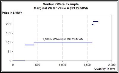
Offers for hydro systems in EMarket reflect more than just the marginal water value. For example, a set of offers for the Waitaki system, shown at right, during a week when the water value is $99.29/MWh could be structured as shown in Figure 17. There are 5 offer bands priced from $1/MWh up to $215/MWh, but only the third band of 1,180 MW is priced at water value, which is the value of water in the seasonal storage reservoirs Lake Pukaki and Lake Tekapo.

Band 1 reflects the need to satisfy the must run requirement of 120 cumecs at the Waitaki power station. However, this requirement only amounts to about 20 MW at the Waitaki dam, so the rest of the band is a reflection, in this particular instance, of all the water moving through the complex Waitaki river chain to satisfy the minimum flow constraint.

The second band in this example is 180 MW at $87/MWh and in this particular case is a reflection of the water value of Lake Tekapo relative to Lake Pukaki.

The fourth and fifth bands are priced at $199/MWh and $215/MWh, respectively, and are most likely a reflection of the need to spill past some stations, reducing the overall efficiency of the Waitaki system, when output goes above 1,600 MW.

Figure 18 - Waitaki Hydro System

The number, size and price of these offer bands varies during each simulation run with EMarket as the water value changes and as the distribution of water within the Waiatki river chain changes. When Waitaki is dispatched, EMarket ensures that the movement and storage of water along the river chain is correctly updated. In this way, the behaviour of each of the major hydro systems can be modelled with some considerable detail in EMarket.

This can be seem most dramatically when detailed simulations are run for the driest of years. During winter nights, when demand is low and the HVDC is expected to transfer power southward, conserving southern hydro storage, EMarket will offer the Waitaki system in such a way that often only 20 MW is generated on this system which normally generates at over over 1,000 MW. This is explained by the extremely high value of water in these instances. However, EMarket satisfies the 120 cumecs must-run constraint at the Waitaki power system, the last in the chain shown in Figure 18 by pricing water in the small lake behind this power station just low enough for it to be dispatched. We have confirmed with Meridian Energy that this level of generation is possible, though only likely in the event of a sever drought and low storage.

A refinement on EMarket's basic hydro offers is provided by the optional "STRCO" feature, standing for Short Term River Chain Optimisation. The STRCO option performs a dynamic programming optimisation on offers from stations along the entire river chain, with the water value as a key input.

Hydro stations in a hydro system may be configured by the user to have their own, individual injection nodes, in which case EMarket distributes generation along the nodes in the hydro system, as described in detail in section 8.2.

EMarket does not take account of market power when calculating water values, ie it assumes all hydro generators offer at their marginal water value without using market power. EMarket provides other, more flexible facilities for the user to model and experiment with the use of market power, for example the optional Company Optimisation feature which optimizes gross profit across all generators, hedges and retail load modeled for a generating company. Effectively, EMarket calculates water values in the same way as a centrally planned utility would if they assumed the modelled thermal offers used in the calculations were actually marginal costs for those generators.

Distribution of Hydro Offers Over Multiple Nodes

In versions of EMarket distributed prior to February 2006, all generation from any given hydro system was offered at one node on the grid, and dispatched at that same node. The node could be chosen for each hydro system. For example, all Waitaki offers and dispatch were typically configured by the user at Benmore and Whakamaru for the Waikato hydro system.

In order to improve constraint and locational pricing modelling, EMarket was upgraded early in 2007 to model the distributed injection of this generation at each station in their respective hydro system.

Overview

In the New Zealand electricity market the hydrological constraints under which stations in a system operate are not modeled in the market dispatch engine, SPD. Offers for a large hydro system are made by station, and dispatched within SPD as stations. But under the market’s “block dispatch” rules, each hydro system manager may dispatch the stations on their respective hydro system any way they please provided that the total dispatch equals the total of all stations dispatched by SPD (Certain conditions must be met to qualify for block dispatch). This arrangement relies on a certain amount of human judgment, and so to model it requires some assumptions about the aims and methods of the system and grid operators.

These assumptions are made:

• offers for each station will be made so that the redistribution of generation will be kept to a minimum;
• offers, nodal prices and dispatch reflect the effect of transmission constraints as closely as possible;
• offers reflect the optimal operation of the hydro system.

Given these assumptions, the following requirements for EMarket should be sufficient to ensure good modeling of the hydro system within the market:

• generation within a hydro system is subject to all relevant hydrological constraints;
• generation reflects optimal operation given the nodal prices produced;
• generation is subject to all transmission constraints.

The Solution

Each station within a hydro system can have an injection node defined by the user. EMarket creates offers as it always has – refer section 8.1 - first ascertaining optimal operation and the marginal value of water usage given different levels of total generation, then dividing this into bands of significantly different marginal value and creating an offer for each of these. When these offers are dispatched in EMarket they are not associated with a single node, but instead with a distribution across the nodes defined for each station in the system. EMarket then dispatches these distributed offers with regard to all transmission constraints, and calculates power flows on the grid consistent with the distributed generation.

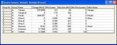
For example, suppose that Table 2 represents optimal generation for the stations in the Waitaki chain at the upper end of four hypothetical price steps.

Table 2 - Example Optimal Dispatch

In EMarket the second offer band brings on generation at TKA and TKB only, accordingly this band will offer 167MW at $7/MWh, with the generation distributed 14% at TKA and 85% at TKB.

Once all offers are dispatched, the dispatched generation relating to each offered band will be distributed across the stations in proportion to the original optimal generation shown in Table 2 as follows:

Table 3 - Example Distributed Offers

Notes for Modellers

1. If the nodes for stations are not set by the user, or do not exist in the grid, then the generation will appear at the default hydro system node.
2. If all stations remain associated with the default hydro system node, the model will run exactly as it used to.
3. There is still only one Generator entity for a hydro system, so the Generator.Generation figures will report the total system generation only. However the individual injection figures can be obtained via the Node.Injection trait – refer to section Table 4- EMarket Parameters.
4. If Node.Injection is output to disk during a run then individual station generation red bars will appear on the EMarket Map, otherwise all generation will still appear at the default system node.

Performance

The impact of running with offers distributed at nodes along a major hydro system on EMarket performance is an increase in run time of around 5%.

Distributed Offers, a Mathematical Description

Distributing Dispatched Generation

Marginal losses and power flows are modelled in EMarket using the ‘DC power flow’ approximation to the full AC power flow, and are calculated using the matrix equations:

[17]

[18]

where y_i is the net injection at node i, z_i the power flow in circuit i, and L the total losses on the grid.

Net injection y_i consists of total injection at the node, I_i, nodal demand D_i and nodal losses l_i. The nodal losses are actually incurred in the lines but since they are not modelled explicitly in the DC power flow they must be calculated from the power flows once these are known. They are then added back into nodal demand, so l_i is actually the sum of the losses on incoming lines to a node (Some DC power flow models split the losses on each line in two and add each half to the upstream and downstream nodes on the line. The process of calculating the losses is iterative in EMarket: first power flows are calculated, then the accompanying losses. These are added back to nodal demand and the power flows calculated again, etc. This process is stable and converges quickly):

[19] y_i = I_i - D_i - l_i

Injection I_i is a function of the dispatch of each offer made at node i, and is normally calculated by adding the dispatch of each offer to give total injection. This can be expressed in a matrix equation using a distribution matrix K:

[20]

where g_m is the dispatched generation for offer m, and K_im = 1 where offer m is at node i and 0 otherwise. Hence rewriting injection I_i in terms of the K matrix allows us to formulate the power flow in terms of the generation dispatched in offers at node i.

In order to distribute offers, a simple adjustment is made to the K matrix in equation [20]. If offer m is distributed over a set of nodes S then

a) 0 < K_im < 1 for each node i in S, and

b)

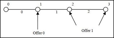
For example, if offer A is located at node P, and offer B is distributed equally between nodes P and Q then the K matrix will be:

	A	B
P	1	0.5
Q	0	0.5

Applying equation [20] with the adjusted K matrix will result in dispatch equations that model offered generation as being proportionally distributed over two or more nodes.

The dispatch power flow equation

During the dispatch process a matrix formula is constructed that calculates power flow as a function of dispatch:

[21]

where is the base power flow resulting from demand and nodal losses across the grid and g_m is the generation dispatched from offer m. This formula is a combination of equations [17], [19] and [20], with:

[22]

[23]

Equation [21] now expresses the power flows in terms of dispatched generation by offer rather than by node.

Figure 19 - A Simple Network Example

The H’ matrix is constructed from the H matrix and the nodal allocations of the offers. With normal, non-distributed offers each column m of the H’ matrix is copied from a column i of the H matrix where i is the node at which offer m is made. With distributed offers though the associated column is a linear combination of columns from H.

In this simple network one offer is made at node 1, the other is distributed evenly between nodes 2 and 3. All lines have equal impedance (although this does not effect the H matrix in this simple case). Using node 0 as the swing node, the power flow matrix H is:

	Node 1	Node 2	Node 3
Line 0	1	1	1
Line 1	0	1	1
Line 2	0	0	1

H' will then be:

	Offer 0	Offer 1
Line 0	1	1
Line 1	0	1
Line 2	0	0.5

Water value Location Adjustments

As noted in section 6.7 there are significant differences between the full simulation runs and the coarser simulations undertaken just to calculate water values, the treatment of losses being a case in point. Another important difference is that water value simulation grid is treated as “flat” in respect of nodal prices, i.e. there is only ever one price in each island. This occurs because losses are assumed constant and the only grid line modelled is the HVDC link.

In the full simulation runs, however, losses are calculated dynamically, and dispatch and pricing are fully nodal, based around a grid which typically has 180 nodes and about 200 lines. The resulting prices vary by node and are anything but flat – large price differentials and reversals constantly occur.

The impact of full nodal pricing on the accuracy of the full simulation runs would be quite large if the water values were not adjusted for changes in the relative pricing across the grid, although this adjustment is an option under the control of the user. Assuming the adjustment is turned on, the water values for each hydro system are adjusted at each dispatch in the full simulation to bring them back in line with the thermal offers represented by the water value contours.

For example, suppose Waitaki storage is sitting on the contour for the simulated $60/MWh offer relating to the second unit at the Huntly power station in the North Island, and that power is transferring north on the HVDC link. All other things being equal, we would expect the Waitaki to be offered at $60/MWh. However, nodal pricing with power flowing generally north from the Waitaki right up to Huntly will introduce a significant price differential, let’s say 10%, in favour of Huntly. Therefore if Waitaki offers at $60/MWh then it will not be dispatched as much as it would have in the simulations for calculating water values. The water value adjustments therefore take into account these differences – in this case Waitaki would offer 10% less than the $60/MWh water value, or $54/MWh.

The water value adjustments are capped at 1.5 times the original water value because lowering raising the price in the presence of a line constraint on the grid, which can produce very large price differentials, would not achieve anything in terms of altering the dispatch of the hydro system.

These adjustments might seem coarse at first sight and one might ask – why do the water values not take account of nodal pricing and dispatch? Apart from the obvious response that this would significantly slow down the production of water values, if we consider the problem of how to minimise fuel burn in a centrally planned utility, then we can see that the quantities of hydro dispatched are critical, not the prices at which the hydros are offered. We saw in section 5.2 that maximising revenue requires the same strategy as minimsing total fuel burn when we ignore market power, so once again we can see that preserving the optimum quantities is paramount – this is exactly what the water value adjustments do.

EMarket Hydro Parameters

Hydro generators are modelled in EMarket in considerable detail, as indicated by Figure 20 which shows the input screen for stations on the Waitaki system. Each station is given a name and can have a storage lake and tributary inflows associated with it. The basic station parameter is the maximum generation in MW and the MW per cumecs value which is used to convert water flow release to generation.

Stations may also have a minimum flow requirement immediately downstream.

Figure 20 - Hydro Station Parameters

Reservoirs may be grouped together in the generic model – this will simplify the model somewhat and improve performance. When this is done the grouped reservoirs are modelled as one reservoir, although the model will still show input and output values for all reservoir in the group.

To allow the user to model more complex river chains, two additional station parameters can be set via the EMarket Schedule (described briefly in section 10):

• MinGen – minimum generation at the station;
• Diversion – a flow in cumecs which must be diverted around the station at all times, for example the diversions around the Aqua stations proposed by Meridian Energy.

Since most of the station parameters are accessible in the EMarket Schedule, the user is able to model such events as parameters that change over time or in response to particular events.

The following figure shows the generic serial hydro system model currently used.

Figure 21 - Generic Hydro Model

List of Parameters

The following table shows the range of parameters that are available in EMarket for the user to interrogate or change at run time. Parameters marked with the following denote restrictions on the ability of the user to change the value of the parameter at run time:

# = Read only: derived at run time

## = Read only at run time obtained from an adjustable input file (e.g. nodal demand)

^ = Static value (user defined but cannot be changed at run time)

Table 4 - EMarket Parameters

Name	Unit	Formula or From
Nodes
Node.Injection#	MW	; where Generator.Node = Node
Node.Price#	$/MWh	Dispatch Price Engine (DPE)
Node.LocalDemand##	MW	Demand Profile and Regional Demand
Node.Demand	MW	L(1+LR/V0); WhereL=Node.LocalDemand; R= Node Resistance; V0 = Base Voltage
Generators
Generator.Outage		Input: b/w 1 or 0; Schedule
Generator.CurrentCapacity	MW	Max Ouput*(1-Generator.Outage)
Generator.Generation#	MW	DPE
Generator.Cost#	$/Hr	; Where OfferBand.Generator = Generator
Generator.Efficiency	%	input
Generator.Revenue#	$/Hr	Generator.Node.Price * Generator.Generation
Generator.DispatchFR#	MW	DPE
Generator.DispatchSR#	MW	DPE
Generator.ReserveCost	$/Hr	DPE (Non static trait)
Generator.NonFuelMC	$/MWh	=Generator.Cost($/Hr)/Generator.Generation(MW) (input, for major hydroSystem only; Non static trait)
Generator.CommDate		Input
Generator.MothDate		Input
Generator.UnitSize		Input
Generator.RSlope^		Input (available when reserve dispatch is modelled)
OfferBand
OfferBand.InitPrice	$/MWh	Input: Direct tab: P<br\>For HydroSystem and HydroStation: Hydro Modal
OfferBand.InitQuantity	MW	Input: Direct tab: Q
OfferBand.Price	$/MWh	= Offerband.InitPrice; except where using Company Optimisation
OfferBand.Quantity	MW	Input: Quantity Profile tab
OfferBand.MarginalCost	$/MWh	Input: Direct tab: MC (Default: = OfferBand.InitPrice)
OfferBand.Dispatch	MW	DPE
OfferBand.Cost	$/Hr	OfferBand.Dispatch * OfferBand.MarginalCost
Line
Line.Capacity	MW	Input: +Limit; Schedule
Line.RevCapacity	MW	Input: -Limit; Schedule
c	MW	DPE
Line.Separation (Line.LM)	$/MWh	DPE
Resistance^	Ω	Input
Reactance^	Ω	Input
Fixed losses	M	Input
Reserve Regions
ResRegion.RAFFR		Input: RAF FR
ResRegion.RAFSR		Input: RAF SR
ResRegion.BaseRisk	MW	Input: Base Risk
ResRegion.ImportSubtractor	MW	Input: Import Risk Subtractor
ResRegion.PriceFR#	$/MWh	DPE
ResRegion.PriceSR#	$/MWh	DPE
Company
Company.RetailCost#	$/Hr	; Where Node ∈ Company
Company.RetailLoad	MW	Where Node ∈ Company
Company.RetailRevenue#	$/Hr	Where Node ∈ Company
Company.ContractQty	MW	Where Node ∈ Company
Company.ContractRevenue#	$/Hr	Where Node ∈ Company
Company.Generation#	MW	Where Generator ∈ Company
Company.GeneratorCost#	$/Hr	Where Generator ∈ Company
Company.GeneratorRevenue#	$/Hr	Where Generator ∈ Company
Company.GrossProfit#	$/Hr	Company.RetailRevenue + Company.ContractRevenue + Company.GeneratorRevenue – Company.RetailCost – Company.GeneratorCost
HydroStation
HydroStation.MaxStorage	Mm3	Input:Storage
HydroStation.MWperCumec	MW/CM	Input: MW/cumec
HydroStation.MaxGen	MW	Input: Max Gen
HydroStation.MinFlow	m3/s	c
HydroStation.MinGen	MW	Input: Schedule
HydroStation.Diversion	m3/s	Input: Schedule
HydroStation.HydroStorage#	Mm3	Hydro Model
HydroStation.HydroMWV	$/CMH	Hydro Model
HydroStation.HydroRelease	m3/s	Hydro Model
HydroStation.HydroSpill#	m3/s	Hydro Model
HydroStation.Inflows	m3/s	Hydro Model
HydroSystem
HydroSystem.SystemStorage#	GWh	Hydro Model
HydroSystem.SystemMWV	$/MWh	Hydro Model
HydroSystem.SystemRelease	m3/s	Hydro Model
HydroSystem.SystemSpill#	MW	Hydro Model
Region
Region.Demand#	GWh	Input: Schedule
Region.DemandAdj		Input:Schedule
Region.DemandElast		Not on the output list
Region.DemandAct		Not on the output list; Region.Demand*Region.DemandAdj*Region.DemandElast

Highly Constrained Hydro Systems

Some hydro systems, Manapouri for example, are highly constrained by the requirements of their resource consents. Where these are not capture by water values, the user may also directly alter the offer strategy by modifying some of the hydro parameters shown in the previous section using EMarket’s Schedule.

Multi-year runs

Although not directly related to the detailed modelling of hydro systems, this important feature allows single year runs to be daisy chained together with the final storage from inflow scenario x in run n being used in run n + 1 as the starting storage for inflow scenario x + 1. For example, a series of 10 runs can be set up to model a full decade with 1931 scenario final storage in the first year giving the start storage for 1932 in the second year, and so on.

Prior to this enhancement, multi-year runs could be set up but water values were not updated each year. Single year runs could only be linked with considerable manual intervention, but this enhancement makes the linkage automatic, with new water values calculated for each year.

Impact of Spill Penalties

The discussion of how water value contours are calculated up until now has used zero as the value of an additional unit of water arriving in an already full reservoir. But currently in New Zealand the major generators are required to report any and all spill, with the possibility of excessive or unnecessary spill attracting, at the least, negative publicity. EMarket allows the user to enter a spill penalty value for each major reservoir, which has the effect of making the value of an extra unit of water in an already full reservoir less than zero, i.e. it incurs a cost equal to the input spill penalty value.

The user may wish to enter a non-zero spill penalty if the reservoir is averse to spilling, for example, as many are in New Zealand given that all spill must be reported. This is recognised in the calculation of N_c at equation [14], noting that the equation for P_c is now

[**]

where C_spill is the spill penalty entered by the user for each hydro system.

The impact of a spill penalty is to lower contours that are nearer to the top of the reservoir, thus lowering the hydro’s offer earlier (than it would with a zero spill penalty) as the risk of spill rises. Referring to Figure 6, the scenarios hitting the top of the reservoir, being counted at C_spill and not at zero, will reduce the calculated average of all scenarios, lowering the MWV of the point represented by S₁ at T₁. Since this is already a contour, let’s say at price P_c, P_c will now exceed the calculated MWV, so the position of the contour will need to lower so that P_c and the calculated MWV are once again the same. The amount of the lowering will depend how many forward projections hit top, so the impact on water value contours will be greater on lower priced contours than on higher priced contours.

Other Features

This section provides a brief list of other important features in EMarket.

Nodal Dispatch and Pricing

For use in New Zealand, EMarket dispatches generation offers at each step in the full simulation (Not the simplified weekly dispatch used in the simulation phase of water value calculation) using the methodology contained in the Electricity Governance Rules which specify that dispatch and pricing should take into account losses, line constraints and instantaneous reserves. EMarket’s “IQP” dispatch and pricing algorithm has been benchmarked against the SPD model used by the System Operator and Pricing Manager to dispatch and price generators and electricity in the wholesale spot market.

Instantaneous Reserves

EMarket allows generators to be set up to offer reserve and these offers are dispatched along with energy offers by EMarket’s IQP dispatch and pricing algorithm.

Grid Modelling

The grid modelling in EMarket may contain all approximately 450 nodes and 800 lines and transformers modelled in SPD. In practice, however, highly accurate results are obtained with an aggregated grid of about 180 nodes and 200 lines, with a consequent benefit in reducing the time taken for each dispatch.

This level of detail allows the users to obtain highly accurate nodal prices, power flows and line constraint information from EMarket simulation runs.

Demand Modelling

EMarket can run at resolutions from half hourly up to weekly. Because of this, it accepts demand data in a half hourly format. Demand profiles can be updated annually, for example, based on actual demand data. Users can set up their own demand regions on the grid and set the EMarket Schedule up to vary demand in each region separately to demand in the other regions. This provides the user with a high degree of flexibility in modelling demand over extended periods as demand grows, for example.

Thermal Generators

Thermal generators offers may be setup in a number of ways in EMarket. For example, they can be set up on a static time-based schedule where they change quantity and/or price at specified dates.

Or they can be manipulated in complex ways in the EMarket Schedule, or offered as a fixed profile at a specified price. They can even be linked to internal Monte Carlo models of fuel prices to simulate how offers might change over time with natural gas, coal or oil prices, for example.

Monte Carlo Fuel Prices

This facility allow fuel prices to be modelled as varying over time based on a starting price, a process which adds normally distributed noise to fuel prices, and a process which tends to pull fuel prices back to a longer term mean value over time. This approach to modelling fuel prices has received a high degree of attention in the literature in the last few years and has proven to be simple yet effective in a variety of applications.

The Monte Carlo feature uses a mean-reverting model and has recently been applied, as a first approximation, to the modelling of wind farms.

Schedule Programming

The EMarket Schedule is effectively a simple programming language embedded within EMarket which allows the user to read and change parameters, for example those listed in Table 4 - during full simulation runs. Any new variables created within the Schedule can also be read, changed and output just like the predefined EMarket parameters.

Productivity Enhancements - Outputs and Reports

The user has high degree of control over how much output data is saved from each full simulation run, and how the saved data is formatted in summary reports. Given the large amount of data (The user is actually free to set the outputs they actually want to save and this can be quite minimal) that EMarket may produce, the ability to list and/or summarise certain data into customised files which are easier for the user to work with, is of great benefit.

Productivity Enhancements - Time Resolutions

Users have a high degree of control over the resolution of each full simulation run – half hourly up to weekly may be specified. Furthermore, modes can be mixed, e.g. a run may proceed in a weekly mode until a specified date at which point it switches to half hourly – an advantage if half hourly values are only required for a short period but the user wishes to have the simulation run execute at great speed.

Company Optimisation

The user may define companies within EMarket which own generation, and have retail load and hedging contracts. Company optimisation can be turned on for a company so that it optimises gross profit given its generation and retail portfolio. This feature provides a way for the user to investigate, for example, how a large hydro generator might vary its offers away from water value by using market power.

STRCO

The Short Term River Chain Optimiser can be turned on for each major hydro system. This is a dynamic program which optimises offers for each major hydro taking account of current market prices and the detailed characteristics and constraints in the river chain.

Back to Water Values Technical Bulletins