Difference between revisions of "EMK:Multi Dimensional Water Values"
| Line 151: | Line 151: | ||
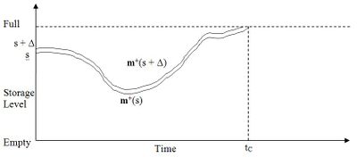
where t<sub>c</sub> is the point of convergence. This means that marginal benefit only needs to be measured up to this point of convergence as it will be zero from that point on. This process is illustrated in Figure 7. | where t<sub>c</sub> is the point of convergence. This means that marginal benefit only needs to be measured up to this point of convergence as it will be zero from that point on. This process is illustrated in Figure 7. | ||
[[File:MDWV Figure 7a.jpg|400px|thumb|centre|Figure 7 - Conversion of Projected Storage Trajectories]] | [[File:MDWV Figure 7a.jpg|400px|thumb|centre|Figure 7 - Conversion of Projected Storage Trajectories]] | ||
| + | |||
| + | Figure 7 shows trajectories originating from storage points s and s + ∆ and converging when the higher trajectory is forced to spill when storage is full. Of course the market statuses contain many other factors, including the storages of all other reservoirs, so this is a very simplified diagram. However it does illustrate the factors involved in calculating marginal benefit. These factors are: | ||
| + | #To a certain degree the only difference between '''m'''<sup>+</sup><sub>t</sub>(s) and '''m'''<sup>+</sup><sub>t</sub>(s + ∆) is the difference in storage at reservoir r, and this difference may not change greatly until storage is constrained at full or empty; | ||
| + | #Release, and therefore generation, of parallel storage paths in reservoir r will be the same, so the benefit from generation will be equal until convergence; | ||
| + | #When storage is constrained at full, and spill occurs, the difference in benefit from generation will be zero; | ||
| + | #When storage is constrained at empty, the difference in benefit from generation will be the energy price in the step where convergence occurs. | ||
| + | |||
| + | Subject to the reservations listed below then, it appears marginal benefit can be calculated by finding the point of convergence and measuring it just at that point. If it is at a full point the marginal benefit is zero; if it is at an empty point marginal benefit will equate mostly to the energy price at the time of convergence. | ||
| + | |||
| + | Some reservations to consider when applying this method are: | ||
| + | #There may be some additional penalty required for spilling water under some circumstances, to allow for the environmental, commercial or reputational risks involved, for example; | ||
| + | #Some levels of storage may be deemed undesirable in themselves, for reasons such as flood risk control, dust problems, loss of head or reputational risks; | ||
| + | #Trajectories will generally converge at a certain rate even when storage in not constrained, because marginally higher levels tend to make slightly cheaper energy offers; | ||
| + | #The marginal benefit from generation also includes its effect on energy price in general and the benefit or loss incurred by the rest of the operator’s portfolio by this change in price. | ||
| + | |||
| + | These reservations are left out of the description for now and dealt with in the Appendices. The primary method used here for finding marginal benefit, and therefore water value, is projection to a storage constraint. | ||
| + | |||
| + | ===Calculation of Water Values=== | ||
Revision as of 15:42, 26 November 2012
Scenario Projection Modelling for Stochastic Water Valuation in EMarket
Disclaimer
Reasonable care has been taken to ensure that the information in this paper is up to date at the time of issue. Potential users of EMarket should, however, ensure that they evaluate EMarket and this paper through an appropriate evaluation process in consultation with Energy Link. The authors are also reliant on certain information external to EMarket and Energy Link, for which no liability or responsibility can be accepted.
Introduction
This technical bulletin is intended to provide users and interested parties with a detailed explanation of how EMarket’s multi-dimensional (MD) water values are calculated and applied. EMarket was designed as a market simulation model rather than as an operational model and the algorithm developed by Energy Link for use in EMarket was designed to give a high degree of accuracy at high speed for this purpose. Speed of operation is a strength of EMarket and ensures that users can turn new or modified simulations around quickly, achieving high levels of productivity.
EMarket4 replaced EMarket3 which used two-dimensional (2D) water values. A 2D water value for reservoir A is calculated with reference to time of year and to storage currently in reservoir A. MD water values in EMarket are calculated with reference to time of year, storage in reservoir A and storage in all other reservoirs (i.e. they are 3D water values). MD water values therefore take account of total storage, and recognise the fact, for example, that when storage in reservoir A is low, future market outcomes may be different depending on whether total storage is either high or low. The behaviour of MD water values relative to 2D water values is briefly explained in: Water Values and Hydro Offers.
EMarket is now set up to allow the user to switch between MD and 2D water values, ensuring backward compatibility.
The water values have also been rewritten in EMarket to make future enhancements easier to implement. For example, water values in Pukaki could be enhanced to take account of time of year, storage in Pukaki, storage in Tekapo, and all other storage (4D water values). Or water values could take account of contract position, market power, or uncertainty in demand, for example.
This document is divided into three parts. Section 3 outlines the scenario projection method and its application in EMarket. Section 4 describes the mathematic principles behind the method is a more thorough manner.
Summary
When water values have been calculated using the projection method described in this bulletin, and applied to the operation of hydro plant, they should be valid in the following sense:
Given that the scenarios modeled are considered to be representative of expected market conditions, and that the inputs used in the water value function are representative of the values considered when evaluating water value, then the marginal water value produced by this method will reflect the expected marginal value of that water.
MD water values currently use time of year, local storage, and total of all other storage to calculate and to look up water values in each major reservoir. This method is an improvement over 2D water values which made strong assumptions about how storage evolved across all reservoirs. These assumptions have been relaxed in MD water values so at each time step storage in other reservoirs can take on values other than those assumed in 2D water values. As a result, MD water values produce model outputs which are more consistent with actual market outcomes.
An important feature of the EMarket MD method is that it is able to allow for serial correlations in market scenarios, regardless of the form that such correlations might take. This avoids the need for the statistically based corrections applied in some other models. Serial correlations are not only important for individual reservoirs, but their impact on the market will also be affected by correlation of inflows between different catchments. Other statistical properties such as wind flow correlation can also be captured provided realistic sets of scenario can be generated.
Scenario Projection Modelling in Practice
This section aims to give a general overview of how scenario projection is applied to water valuation.
General Principles
The underlying meaning of water value relates to the decision to use water for generation at any given time. This decision involves comparing the immediate benefit accrued by using the water with the benefit of holding it for future use. Water value can be defined as expected future benefit that a small, or marginal, amount of extra storage would confer in this situation. Determining this value is a stochastic process because of the unpredictable elements affecting future operation, especially the variability of reservoir inflows.
The expected benefit of a marginal amount of storage is normally only easily determined in situations where reservoir storage is constrained. When the reservoir has reached its upper limit and storage cannot be reduced operationally, this marginal value is nominally zero – the extra water confers no benefit. When the reservoir reaches empty, and operational guidelines force all available water to be used, the marginal value is equal to the immediate value of using the water.
When the reservoir is unconstrained the marginal value is harder to determine. As well as requiring a good model of the stochastic elements of the market, a number of subtle assumptions need to be made about the relationship between estimated water value and hydro system operation.
The usual methods of solution for this problem all involve iteration. The reason for this iteration is a circular relationship between a chosen set of water value guidelines and the expected benefit that results from using those guidelines. In a very simple form this relationship could be summarised as:
- Water value guidelines too low → Water use and Generation Higher → Greater likelihood of shortage → Higher expected marginal benefit.
- Water value guidelines too high → Water use and Generation lower → Lower likelihood of shortage → Lower expected marginal benefit.
So, in a very simple sense, expected marginal benefit is an inverse function of water value. The purpose of iteration is to find the point where the values are equal. Of course the water value guidelines and expected marginal benefit are not single values, but functions of storage levels and time. The method of iteration is in principle the same, only significantly more complicated, as an iterative method for solving a single dimensional function such as the bisection or Newton-Raphson method.
Given that iteration is to be used to find optimal water values, the next important step to decide is how expected marginal benefit can be calculated from a set of water value guidelines. This is covered in the next section.
Calculation of Expected Marginal Benefit
The stochastic nature of the hydro system’s operating environment is modeled by generating a finite set of equally likely future situations from any given starting situation. The marginal benefit of storage can then be calculated by taking the average of the marginal benefit values in all the future situations. This method creates a number of future problems from a single current problem and usually requires some sort of ‘back projection’, that is an initial guess at a set of values in the distant future and the repeated calculation of values in discrete time steps that work back from that time. For a cyclic solution, such as one for seasonal hydro operation, this method can be viewed as an iterative one that converges after a certain number of iterations, rather than one that returns from a far distant date.
One of the primary problems of back projection lies in its step-wise nature. It can be very difficult to model features of the environment that extend beyond the period of one step. One particular bug bear of water value modelling is the serial correlation of inflows: it is unrealistic to regard them as independent from one step to the next. Simple analysis of inflow data shows that inflows can actually correlate over long periods, for example during an event resulting from a medium term climatic event.
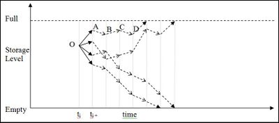
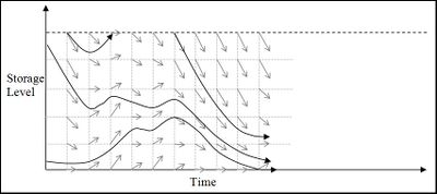
The method used here was developed with the aim of encapsulating the challenging statistical nature of inflow modelling. With this aim in mind a significant shift has been made in the philosophy behind the back projection method. Marginal values are thought of as being the result of evaluating marginal benefit along a projected path for as long as marginal benefit would be realised along that path. Conceptually this involves following paths until they reach a point of storage constraint. The paths follow the progression of storage as it would occur for the scenario with the water value guidelines in place. In Figure 1 the water value at the point O at time ti is evaluated using four scenarios. If back projection were used the resulting value would be determined from the four values at time ti + 1. With scenario projection the value results from the zero values where two paths reach full storage and the shortage values where two paths meet empty.
These scenario projections are never actually performed, but the same result is achieved by using back projection and adding the simple expedient of calculating values separately for every scenario. In the diagram the expected marginal benefit calculated at point A is back projected from the point B only (because this point results from applying the same scenario) and likewise comes in turn from points C and D. The marginal benefit at D results from a projection that arrives at full, so all the values A to D are zero. Bear in mind here that these values are the marginal benefits for only one of the scenarios. Only when it is time to calculate overall expected marginal benefit are the values from the scenarios combined to give one figure for each point in the storage-time space.
The marginal value of water at either full or empty is of fundamental importance in calculating water values. Consider a “thought experiment” concerning a hypothetical reservoir of infinite storage. In this case there is no full and no empty, and so the future value of water is irrelevant. Put another way, there is no trade-off to be made between releasing now or later, as there will always be more than enough water to release any time in the future. Hence, in this case water values would be irrelevant and the reservoir owner would offer and generate in a way which simply maximised the generation revenue at each time step.
But real reservoirs are not finite, and do have upper and lower storage constraints: it is the presence of these constraints that requires the present and future value of water to be traded-off, and which in turn creates water values as the opportunity cost of the reservoir being constrained in future.
Extra Dimensions
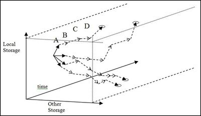
Figure 1 illustrates projection of a scenario where one storage volume is traced over time, but the same concept can be applied where more than one storage value is traced. This means water value profiles can be generated that return water values given the time and multiple measures of the storage situation. The default method chosen for EMarket uses two storage values to determine water value at any time: the storage in the reservoir for which water values are being generated and the total (energy) storage in all other reservoirs in the market. This means projection is done over a three dimensional space, or 3D water values.
Figure 2 illustrates how the scenario projection in Figure 1 might appear with an extra storage dimension.
While 3D water values are used in EMarket (time, local storage, other storage) the process of calculating water values will be illustrated below using only two dimensions (time, local storage) to simplify the visualisation of the process.
The Calculation Process
The following steps illustrate the marginal value calculation process, starting with a set of water values.
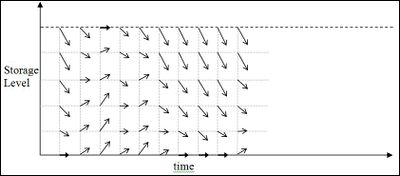
For each scenario the progression of storage from each of a set of sample points is calculated by simulating the market starting at that point. For example, if the point represented a local storage level of X and another storage level of Y at time T, the reservoirs are set to these levels (with other storage will be proportionally allocated). Water values calculated are for this configuration using the current water value profile, with offers generated given the time and the calculated water values, and dispatch calculated accordingly. The resulting storage configuration for the following step is then recorded:
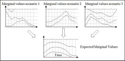
The expected value (for this scenario only) is calculated by assigning a value to all the constrained paths (shown as thick arrows) and back projecting all the others. In the figure below, the regions between the thick black lines will have similar values because they are back projected from areas with similar storage-constrained marginal values.
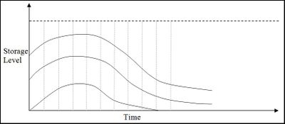
All the scenario marginal value sets are averaged to produce an overall expected marginal value set, as illustrated in Figure 6 below.
This combined set of expected marginal values is then used to adjust the water values by calculating a weighted average of the two values, after which the process is repeated. The values are found to converge reliably by using a weight for the new marginal values that diminishes at each step.
For simplicity, the examples above show water values as a function of time and a single storage value (as in EMarket3), but the process is extended in EMarket gives water value so that water values are a function of time, storage at the reservoir in question and total storage in all other reservoirs. The water values for all large reservoirs need to be calculated at the same time, as the water value profile for each reservoir effects the operation of all other reservoirs. This means the marginal expected benefit is calculated for all reservoirs and then all water value profiles are updated in each step.
Operating Considerations and Adjustments to Marginal Values
The process of calculating expected marginal water value needs to be adjusted in some cases for operating considerations other than the simple storage constraints at empty and full. This is done in EMarket using three adjustment factors: spill penalty; high storage buffer; and low storage buffer.
Spill Penalty
Spill penalty aims to factor in the undesirability (for example, there may be an indirect cost associated with spill) of spillage by allowing the user to assign a negative benefit to the amount of water being spilled in any situation. When marginal benefit is calculated this negative value is given to projections that result in spill. The spill penalty also sets a minimum marginal value for water at any level, since the option to spill this water is assumed to always exist.
High Storage Buffer
This value represents an aversion to allowing storage to exceed a given level, for any reason. This could be for flood management or other resource consent related reasons. A penalty factor is subtracted from marginal value for each time step the projection passes above this level. The penalty is measured in dollars per week per unit of storage exceeding the buffer level in MWh. In order that this value remains fairly constant it is input as a multiple of the expected average price (which is determined by running simulations during the water valuation process). The high storage buffer may result in negative marginal benefit but this is still limited by the spill penalty value.
Low Storage Buffer
This value represents an aversion to allowing storage to fall below a given level. A penalty factor is added to the marginal value for each time period the projection passes below this level. As with the high storage buffer, the penalty is given as a multiple of the expected average price.
Principles of the Scenario Projection Method
Introduction
This section aims to describe in general terms the scenario projection method for determining water value guidelines for hydro generators in a spot electricity market, outlining the mathematical principles being applied and how they relate to best practice by hydro generators.
Expressions and Functional Relationships
Below are some of the fundamental expressions and relationship expressed with the symbols that will be used throughout this section.
Market Evolution
Implicit in the following definitions is an electricity market model that evolves in a series of steps. This could represent the modelling of every dispatch and pricing period in the actual market, but is more likely to be one that models coarser steps such as day-night or week long steps. The step length is undefined here in order to represent all possible models of this type.
Conventions
Symbols defined here can represent single variables or vectors in the natural sense (a subscript indicates a vector index), groups of values with no particular indexing (such as all current market conditions) or functions. The single or vector values will be given lower case variable names, the functions upper case names and the value groups are indicated by bold type.
Definitions
| ti | Time, indexed by step, where ti+1 is the time of the step following ti. |
| mF | Fixed market status. This is the market status not including decision variables – includes date, time, demand, transmission grid, inflows and non-hydro offers, but does not include reservoir storages, water values or hydro offers. ‘Fixed’ refers to the fact that these aspects of the market will be constant throughout the calculations. |
| Sr | Storage by reservoir (r), measured in terms of stored energy |
| Wr | Water value by reservoir |
| OH | Hydro offers |
| m | Complete market status, as at the beginning of a step, including storages and hydro offers |
| m+ | Market step status, includes the prices and dispatched generation for a time step and the market status that results at the end of that time step |
| m+=D(m) | Step transformation: given a market status m this returns the market step status m+ that results for the following step where the market variables have evolved as expected over that period. This is a fixed input to the valuation process and includes pricing, dispatch and hydro operation considerations. |
| w = W(s, t) | Water value function: returns water values for each reservoir given the storages at all reservoirs (s) and the date and time (t). The determination of the function Wr is the aim of the water valuation process. |
| oH=OH(w,s,mF) | Hydro offers function: returns hydro offers given water values, storages and market conditions (inflows in particular). The OH function has a fixed form throughout the water valuation process. |
| m=M(mF,s,W) | Market status as a function of fixed market status, storages and the water value function. Given that OH function is fixed for the valuation process, the function M is also fixed. |
| s'=S(mF,s,W) | Storage step transformation: returns the storages at all reservoirs after an increment of time given the fixed market status, current storages and the water value function. Given that the step transformation is fixed, this function is also fixed for the valuation process. |
| sMAXr | Maximum storage of reservoir r |
Definition of the Optimisation Problem
In this determination of water values the objective is to find the water values for each reservoir that will generate the greatest benefit for the operator of that reservoir. Primarily this benefit will be measured by income from generation, but other factors such as retail commitments and operational and compliance costs can also be factored in. Where possible the description of this water valuation process will refer to ‘benefit’ in the most general terms, to allow for these factors to be considered. The time over which the benefit is measured is not directly defined, but can be considered as an arbitrarily long time period.
Water Values and Marginal Benefit
Water values are generated using a form of marginal analysis, the basis of which is the relationship (Eq. 1):
where ∆ is a small increment of storage and m+t(s) is the market state at time t, given that reservoir r starts with a storage level of s. In other words, the water value is equal to the expected marginal benefit of extra storage in reservoir r (see Appendix 1: Relationship between Water Value and Benefit).
In practice the sets market states m+t(s) and m+t(s+Δ) will tend to converge, so that
- Eq. 2. m+t(s) = m+t(s+Δ) : t ≥ tc
where tc is the point of convergence. This means that marginal benefit only needs to be measured up to this point of convergence as it will be zero from that point on. This process is illustrated in Figure 7.
Figure 7 shows trajectories originating from storage points s and s + ∆ and converging when the higher trajectory is forced to spill when storage is full. Of course the market statuses contain many other factors, including the storages of all other reservoirs, so this is a very simplified diagram. However it does illustrate the factors involved in calculating marginal benefit. These factors are:
- To a certain degree the only difference between m+t(s) and m+t(s + ∆) is the difference in storage at reservoir r, and this difference may not change greatly until storage is constrained at full or empty;
- Release, and therefore generation, of parallel storage paths in reservoir r will be the same, so the benefit from generation will be equal until convergence;
- When storage is constrained at full, and spill occurs, the difference in benefit from generation will be zero;
- When storage is constrained at empty, the difference in benefit from generation will be the energy price in the step where convergence occurs.
Subject to the reservations listed below then, it appears marginal benefit can be calculated by finding the point of convergence and measuring it just at that point. If it is at a full point the marginal benefit is zero; if it is at an empty point marginal benefit will equate mostly to the energy price at the time of convergence.
Some reservations to consider when applying this method are:
- There may be some additional penalty required for spilling water under some circumstances, to allow for the environmental, commercial or reputational risks involved, for example;
- Some levels of storage may be deemed undesirable in themselves, for reasons such as flood risk control, dust problems, loss of head or reputational risks;
- Trajectories will generally converge at a certain rate even when storage in not constrained, because marginally higher levels tend to make slightly cheaper energy offers;
- The marginal benefit from generation also includes its effect on energy price in general and the benefit or loss incurred by the rest of the operator’s portfolio by this change in price.
These reservations are left out of the description for now and dealt with in the Appendices. The primary method used here for finding marginal benefit, and therefore water value, is projection to a storage constraint.
