Company Optimisation in EMarket
Introduction
This technical bulletin is intended to provide users and interested parties with a detailed explanation of how EMarket’s company optimisation feature works.
This paper includes a brief overview of other features in EMarket and a note on enhancements planned in the short to medium term.
Other Documents
This bulletin is one of a series of technical bulletins relating to Energy Link’s EMarket model. Taken together, the bulletins replace the old EMarket User Guide. The full series of bulletins covers an overview of the EMarket model, the details of the four major New Zealand hydro systems modelled in EMarket, water values and hydro offers, power flows, dispatch and nodal pricing, short term river chain optimisation and company optimisation.
Company Optimisation
EMarket is designed to produce stable offering schemes for generation that are, in principle, based on static short or long run marginal costs for each generator. However, when a company owning a generation, retail and hedge portfolio is considered then the optimal offering behaviour for that company as a whole will affect the value of each generation offer. EMarket can now adjust offers to simulate this behaviour, which is called Company Optimisation (CO).
Market Sensitivity
Market sensitivity is loosely defined as the change in price that can be affected by removing or adding generation to the available supply. On an incremental basis, given a supply curve P(s), where P(s) is the price at which a supply of generation s is available, then market sensitivity can be defined as
![]() or the negative derivative of the supply curve.
or the negative derivative of the supply curve.
In practice the supply curve is a lumpy, non-differentiable curve and is not all that useful. In the following analysis we look for more general and approximate relationships between supply and price.
The Supply Curve
Figure 1 is taken from supply curve data over the period of a week from the New Zealand market. For a given price market sensitivity is estimated by first finding the generation available at that price and then finding the price at which 100 MW less generation is available. This shows the average market sensitivity for a range of prices. The average standard deviation is shown by the dotted lines.
This particular week's data indicates that it is possible to estimate market sensitivity (MS) as a linear function of price:
MS = - dP(s) / ds ≈α p
In this case α = 0.005.
The analytical solution to ![]() is P = e-ãs so an exponential fit to the supply curve is indicated.
is P = e-ãs so an exponential fit to the supply curve is indicated.
Company Optimisation Calculators
In the following analysis, location factors are ignored. The problem of optimisation taking location factors into account is considerably more complicated and most of the benefits can be achieved without taking them into consideration, at least for longer term modelling (Optimisation on a short term basis, eg period-by period, is recommended using our EMarketOffer model with its optional Offer Optimiser). The effect of reserve offers is also ignored.
Gross Profit
The gross profit including generation costs for a company in one period (reserve revenue aside) is given by:
π = PEg - μg - PEL + PSL + (PR - PE)*Q
where π is gross profit, g is total generation, PE is the energy price, μ is the costs for generation, L is the retail load and PS is the retail price, Q and PR are the hedge quantity and reference price respectively.
Optimum Gross Profit
With respect to generation, and treating PE as a function of g to account for market sensitivity, the optimum gross profit is given by:
∂π/∂g = 0 =>
dPE / dg * (g - (L + Q)) + PE - μ = 0
Optimum Price/Generation Relationships
Using the Optimum Gross Profit equation, where s0 is the supply without any generation from the company in question.
PE = Exp(α(s0 + g))
dPE/dg = α Exp(s0 + g) = -αPE
which becomes
-αPE * (g - (L + Q)) + PE - μ = 0 or
PE = μ / (1 + α((L + Q) - g))
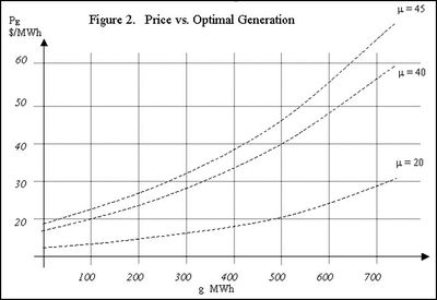
This gives a relationship between price and total generation for optimal solutions, given the marginal cost of generation. Figure 2 shows an example of the optimum price generation relationships for a company with 500 MWh load plus hedges, with a marginal cost of generation at $20/ MWh, $40/ MWh and $45/ MWh. Note that where generation equals load plus hedges, the optimum price is equal to the marginal cost.
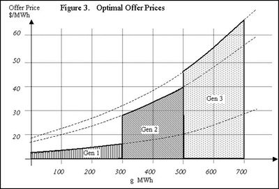
Figure 3 illustrates how the price-marginal cost relationship determines optimal offering. The figure show the optimal offering profile if the company has 300 MWh of generation with a marginal cost of $20/ MWh, 200 MWh at a marginal cost of $40/ MWh and 200 MWh at a marginal cost of $45/ MWh.
This shows that each block of generation will have an offer or offers determined by its marginal cost and the amount of generation with a lower marginal cost. The optimal offer curve for each generation has to be approximated by a number of discreet offers and some compromise between optimality and complexity must be made. For example, to make the simplest possible offers for the generators in figure 3, Gen 1 might be offered at $8/ MWh, Gen 2 at $35/ MWh and Gen 3 at $55/ MWh.
Implementation in EMarket
The implementation of company optimisation in EMarket is based on a variety of modules.
The Supply Curve
At each tick, EMarket determines the market sensitivity by fitting an exponential curve to the supply stack. This is done by running a log-linear regression on the points in the supply curve. Because zero price offers are unable to be fitted to a log linear regression, the regression is not based on 0. Instead the price of all points is first raised by a small base figure.
The log-linear regression provides an expected figure for α for each period of the week. When a run is started α is initialised to 0.0005.
Retail Load and Hedges
These are entered by the user for each company. Hedges follow a schedule and retail load is defined as a proportion of nodal demand for a set of chosen nodes.
Offers
When offers are made for a company using CO, they should be based on marginal cost for all generators. Major hydro systems already offer in on this basis. Once all offers are collected, each company that is using CO is called to adjust its offers. The offers that are made are then adjusted to the optimal offer price for the mid point of the offer. So if μ is the initial price on an offer, g is the quantity of generation offered by the company for less than μ, and g' is the size of the offer then the adjusted offer price is given by:
adjusted offer price = μ / (1 + α((L + Q) - (g + 0.5g')))
The adjusted offers are then entered into the pricing and dispatch process for EMarket.
Size of Offers
Offers are not split and the size of offers is not adjusted by the company optimisation adjustment. This means that large offers may not be brought as close to optimality as smaller offers. The user might consider splitting some of the larger offers made when using CO.


