Distributed Offers from Hydro Systems in EMarket
Aim
Previously EMarket has injected all generation from any given hydro system into one node on the transmission grid. In order to improve constraint and locational pricing modeling EMarket has now been upgraded to model the distributed injection of this generation at each station in the system.
Overview
There is a fundamental difficulty with modeling hydro systems operating in the NZEM. This difficulty arises from the fact that the hydrological constraints under which stations in a system operate are not modeled in SPD. In practice this problem is dealt with by ‘block dispatch’ which allows the system operator to redistribute dispatched quantity within the system. This arrangement is relies on a certain amount of human judgment, and so to model it requires some assumptions about the aims and methods of the system and grid operators.
These assumptions are made:
- Offers for each station will be made so that the redistribution of generation will be kept to a minimum.
- Offers, nodal prices and dispatch reflect the effect of transmission constraints as closely as possible.
- Offers reflect the optimal operation of the hydro system.
Given these assumptions, the following requirements for EMarket should be sufficient to ensure good modeling of the hydro system within the market:
- Generation within a hydro system is subject to all relevant hydrological constraints.
- Generation reflects optimal operation given the nodal prices produced.
- Generation is subject to all transmission constraints.
The Solution
Within the new version of EMarket each station within a Hydro Systems may have an injection node defined. EMarket will then generate offers as it always has - first ascertaining optimal operation and marginal ‘cost’ of water usage given different levels of total generation, then dividing this into bands of significantly different marginal cost and creating an offer for each of these. When these offers are presented to the dispatch engine they are not associated with a single node, but instead with a distribution across the station nodes in the system. The dispatch engine then dispatches these distributed offers with regard to all transmission constraints, and calculates line flows consistent with the distributed generation.
Example:
The following table represents optimal output of the stations in the Waitaki chain at the upper end of four price steps.
| Price $/MWh | TKA | TKB | OHA | OHB | OHC | BEN | AVI | WTK |
|---|---|---|---|---|---|---|---|---|
| 0 | 0.00 | 0.00 | 44.84 | 38.67 | 37.59 | 34.18 | 13.92 | 24.45 |
| 7 | 23.94 | 142.42 | 44.84 | 38.67 | 37.59 | 34.18 | 13.92 | 24.45 |
| 80 | 25.00 | 160.00 | 245.82 | 212.00 | 206.10 | 530.11 | 215.97 | 105.00 |
| 260 | 25.00 | 160.00 | 248.00 | 212.00 | 212.00 | 540.00 | 220.00 | 105.00 |
In EMarket the second offer band brings on generation at TKA and TKB only, accordingly this band will offer 167MW at $7/MWh, with the generation distributed 14% at TKA and 85% at TKB.
Once all offers are constructed they will be distributed as follows
| Price $/MWh | Quantity MW | TKA | TKB | OHA | OHB | OHC | BEN | AVI | WTK |
|---|---|---|---|---|---|---|---|---|---|
| 0 | 193 | 0% | 0% | 23% | 20% | 19% | 18% | 7% | 13% |
| 7 | 167 | 14% | 85% | 0% | 0% | 0% | 0% | 0% | 0% |
| 80 | 1340 | 0% | 1% | 15% | 13% | 13% | 37% | 15% | 6% |
| 260 | 21 | 0% | 0% | 10% | 0% | 28% | 47% | 19% | 0% |
Notes for Modellers
If the nodes for stations are not set, or do not exist in the grid, then the generation will appear at the default hydro system node.
If all stations remain associated with the default hydro system node, the model will run exactly as it used to.
There is still only one Generator entity for a hydro system, so the Generator.Generation figures will report the total system generation only. However the individual injection figures can be obtained via the Node.Injection trait.
If Node.Injection is output then individual red bars will appear on the Map, otherwise all generation will still appear at the default system node.
Conclusion
This distribution of offers is not actually possible under SPD, but it satisfies the requirements set above, and therefore should model actual operations given the assumptions made are valid. Having offers distributed in this way also impacts minimally on the speed of the model, with a slowdown in operation of around 5% only.
Appendix: Distributed Offers, a Mathematical Description
Distributing Dispatched Generation
Marginal losses and power flows are calculated using the matrix equations:
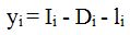
Where yi = net injection at node i, zi = power flow in circuit I, L = total losses. Net injection yi consists of nodal injection Ii, demand Di and nodal losses li (the sum of the losses on incoming lines to a node):
- 3.
Injection Ii is a function of offer dispatch, it is normally calculated by adding the dispatch of each offer to a single node, this can be expressed in a matrix equation using a distribution matrix K:
- 4.
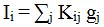
Where gj is the dispatched generation for offer j, and Kij = 1 where offer j is at node i and 0 otherwise.
In order to distribute offers a simple adjustment to the K matrix in equation 4 is made, If offer j is distributed over a set of nodes S then
- a) 0 < Kij < 1 for each node i in S
- b)

For example: if offer A is located at node P, and offer B is distributed equally between nodes P and Q then the K matrix will be:

Applying equation 4 with the adjusted K matrix will result in dispatch equations that model offered generation as being proportionally distributed over two or more nodes.
The Dispatch Power Flow Equation
During the dispatch process a matrix formula is constructed that calculates power flow as a function of dispatch:
- 5.
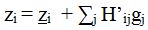
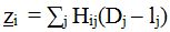
Where ![]() is the base power flow resulting from demand and nodal losses. This formula is a combination of equations 1, 3 and 4, with:
is the base power flow resulting from demand and nodal losses. This formula is a combination of equations 1, 3 and 4, with:
- 6.
- 7.
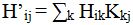
The H’ matrix is constructed from the H matrix and the nodal allocations of the offers. With normal, non-distributed offers each column j of the H’ matrix is copied from a column k if the H matrix where k is the node at which offer j is made. With distributed offers though the associated column is a linear combination of columns from H.
Example - a simple Network

In this simple network one offer is made at node 1, the other is distributed evenly between nodes 2 and 3. All lines have equal impedance (although this does not effect the H matrix in this simple case). Using node 0 as the swing node, the power flow matrix H is:

H' will then be:
